数据来源 https://www.kaggle.com/datasets/ahmeduzaki/global-earthquake-tsunami-risk-assessment-dataset/data
关于此文件 全球地震—海啸风险评估数据集,包含 2001–2022 年间全球范围内 782 次重大地震的地震参数与海啸潜势指标。该 CSV 数据集已预处理为机器学习可直接使用的格式,适用于海啸风险预测、地震分析及地震灾害评估等研究。
主要特征:
•	包含 13 个标准化数值特征(如震级、深度、经纬度等)

•	含有海啸二元分类标签(38.9% 为海啸事件,61.1% 为非海啸事件)

•	数据完整,无缺失值

•	全球地理覆盖范围(纬度 -61.85° 至 71.63°)

•	时间跨度 22 年,涵盖主要地震事件
查看数据 1 2 3 4 import pandas as pd df = pd.read_csv('earthquake_data_tsunami.csv' )df.head()
magnitude(震级)
⸻
cdi(Community Decimal Intensity,公众感受强度)
⸻
mmi(Modified Mercalli Intensity,修订麦加利烈度)
⸻
sig(Significance,事件重要性得分)
⸻
nst(Number of Seismic Stations,地震监测台站数)
⸻
dmin(Distance to Nearest Station,最近台站距离,单位:°)
⸻
gap(Azimuthal Gap,方位间隙,单位:°)
⸻
depth(Focal Depth,震源深度,单位:km)
⸻
latitude(纬度)
⸻
longitude(经度)
1 2 3 df.describe() df.isnull().sum ()
magnitude 0
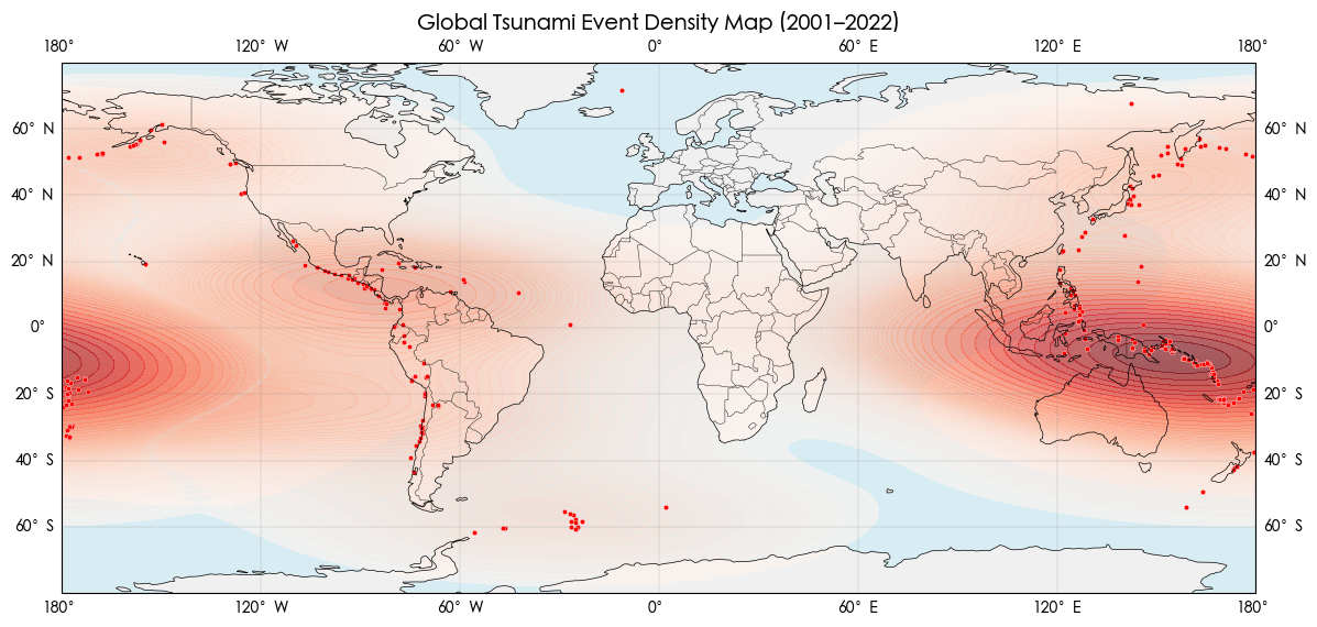
EDA 海啸发生的位置 1 2 3 4 5 6 7 8 9 10 11 12 13 14 15 16 17 18 19 20 21 22 23 24 25 26 27 28 29 30 31 32 33 34 35 36 37 38 39 40 41 import pandas as pd import seaborn as sns import matplotlib.pyplot as plt import cartopy.crs as ccrs import cartopy.feature as cfeature df_tsu = df [df ['tsunami' ] == 1] fig = plt.figure(figsize=(14, 7)) ax = plt.axes(projection=ccrs.PlateCarree()) ax.add_feature(cfeature.LAND, facecolor="#f0f0f0" ) ax.add_feature(cfeature.COASTLINE, linewidth=0.5) ax.add_feature(cfeature.BORDERS, linewidth=0.3) ax.add_feature(cfeature.OCEAN, facecolor="#d8ecf3" ) ax.set_extent([-180, 180, -80, 80], crs=ccrs.PlateCarree()) sns.kdeplot( x=df_tsu["longitude" ], y=df_tsu["latitude" ], cmap="Reds" , fill=True, alpha=0.6, bw_adjust=1, levels=50, ax=ax ) sns.scatterplot( x=df_tsu["longitude" ], y=df_tsu["latitude" ], color="red" , s=10, ax=ax ) ax.set_title("Global Tsunami Event Density Map (2001–2022)" , fontsize=14) ax.gridlines(draw_labels=True, linewidth=0.3, color='gray' , alpha=0.5) plt.show()
从散点图上看 大部份海啸发生的位置处于环太平洋地震带上
说明 海啸的发生与地震发生的位置有关 并且越靠近赤道 海啸发生的频率越高
海啸发生与时间的关系 1 2 3 4 5 6 7 8 9 10 11 df_tsu["Date" ] = pd.to_datetime(df_tsu["Year" ].astype(str) + "-" + df_tsu["Month" ].astype(str) + "-01" ) ts_count = df_tsu.groupby("Date" ).size() plt.figure(figsize=(12,5)) plt.plot(ts_count.index, ts_count.values, color="darkred" , linewidth=1.5) plt.title("Monthly Tsunami Event Count (2001–2022)" ) plt.xlabel("Time" ) plt.ylabel("Tsunami Count" ) plt.grid(True, linestyle="--" , alpha=0.5) plt.show()
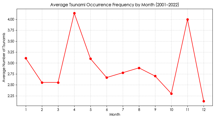
1 2 3 4 5 6 7 8 9 10 11 12 13 14 monthly_count = df_tsu.groupby(["Year" , "Month" ]).size().reset_index(name="count" ) month_avg = monthly_count.groupby("Month" )["count" ].mean() plt.figure(figsize=(10, 5)) plt.plot(month_avg.index, month_avg.values, marker='o' , color='red' ) plt.xticks(range(1, 13)) plt.title("Average Tsunami Occurrence Frequency by Month (2001–2022)" ) plt.xlabel("Month" ) plt.ylabel("Average Number of Tsunamis" ) plt.grid(True, linestyle='--' , alpha=0.5) plt.show()
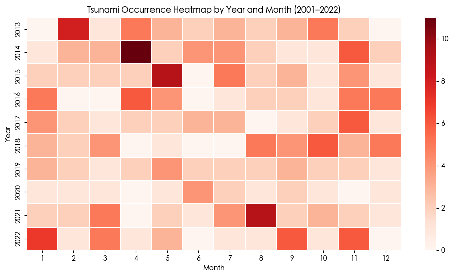
1 2 3 4 5 6 7 8 9 10 11 12 import seaborn as sns import matplotlib.pyplot as plt heatmap_data = df_tsu.groupby(["Year" , "Month" ]).size().unstack(fill_value=0) plt.figure(figsize=(12, 6)) sns.heatmap(heatmap_data, cmap="Reds" , linewidths=0.3) plt.title("Tsunami Occurrence Heatmap by Year and Month (2001–2022)" ) plt.xlabel("Month" ) plt.ylabel("Year" ) plt.show()
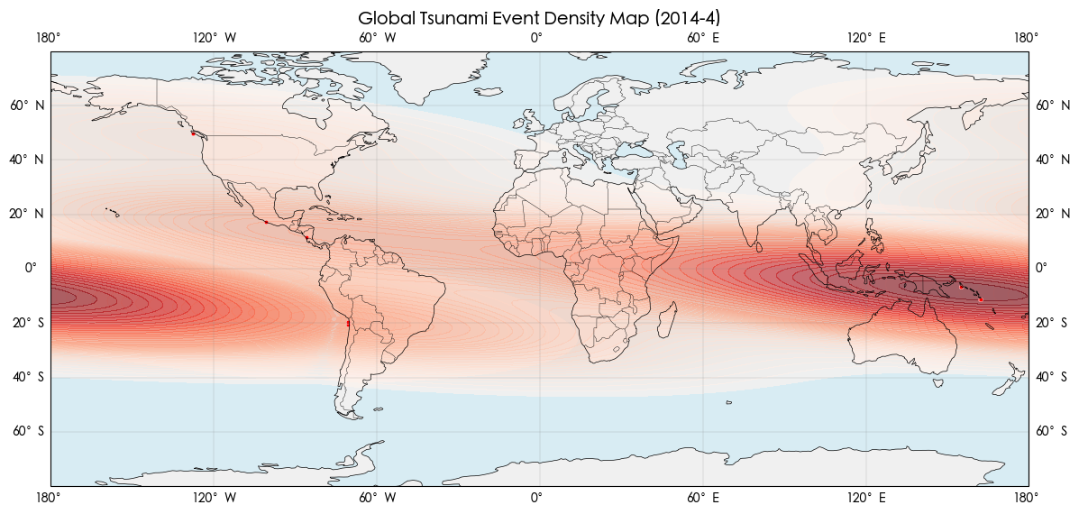
发现 2014年4月海啸数量特别多 查询相关资料后发现 当时智利西北部近海发生了8.0-8.2级的大地震 并且那年处于史上最强厄尔尼诺现象的发展阶段
1 2 3 4 5 6 7 8 9 10 11 12 13 14 15 16 17 18 19 20 21 22 23 24 25 26 27 28 29 30 31 32 33 34 35 36 37 df_2014_4 = df_tsu[(df_tsu["Year" ] == 2014) & (df_tsu["Month" ] == 4)] df_tsu_2014_4 = df_2014_4[df_2014_4['tsunami' ] == 1] fig = plt.figure(figsize=(14, 7)) ax = plt.axes(projection=ccrs.PlateCarree()) ax.add_feature(cfeature.LAND, facecolor="#f0f0f0" ) ax.add_feature(cfeature.COASTLINE, linewidth=0.5) ax.add_feature(cfeature.BORDERS, linewidth=0.3) ax.add_feature(cfeature.OCEAN, facecolor="#d8ecf3" ) ax.set_extent([-180, 180, -80, 80], crs=ccrs.PlateCarree()) sns.kdeplot( x=df_tsu_2014_4["longitude" ], y=df_tsu_2014_4["latitude" ], cmap="Reds" , fill=True, alpha=0.6, bw_adjust=1, levels=50, ax=ax ) sns.scatterplot( x=df_tsu_2014_4["longitude" ], y=df_tsu_2014_4["latitude" ], color="red" , s=10, ax=ax ) ax.set_title("Global Tsunami Event Density Map (2014-4)" , fontsize=14) ax.gridlines(draw_labels=True, linewidth=0.3, color='gray' , alpha=0.5) plt.show()
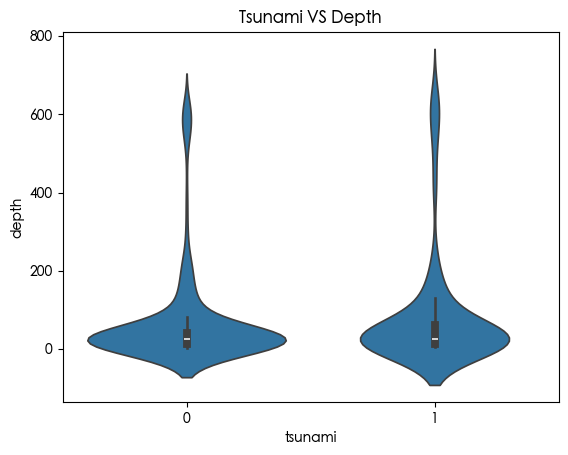
海啸与震源深度的关系 1 2 3 4 5 6 7 import seaborn as sns sns.violinplot( x=df ["tsunami" ], y=df ["depth" ] ) plt.title("Tsunami VS Depth" ) plt.show()
查看数据分布 1 2 3 plt.figure(figsize=(10, 8)) sns.heatmap(df.corr(), annot=True, cmap="coolwarm" , fmt =".2f" ) plt.show()
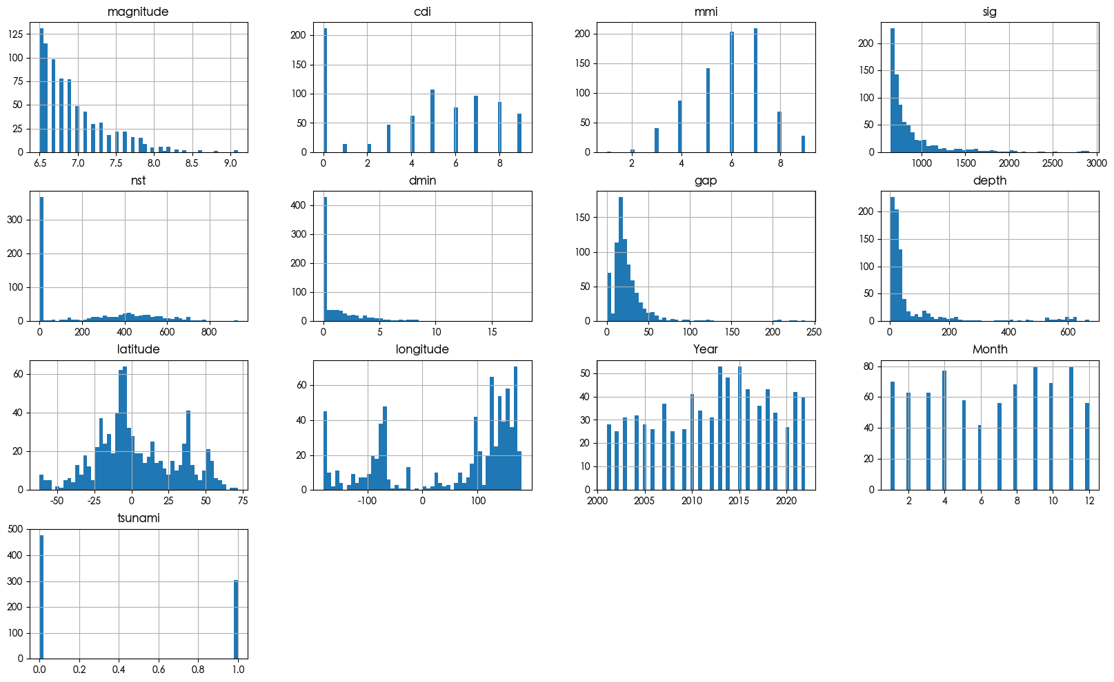
1 2 df.hist(bins=50, figsize=(20,12)) plt.show()
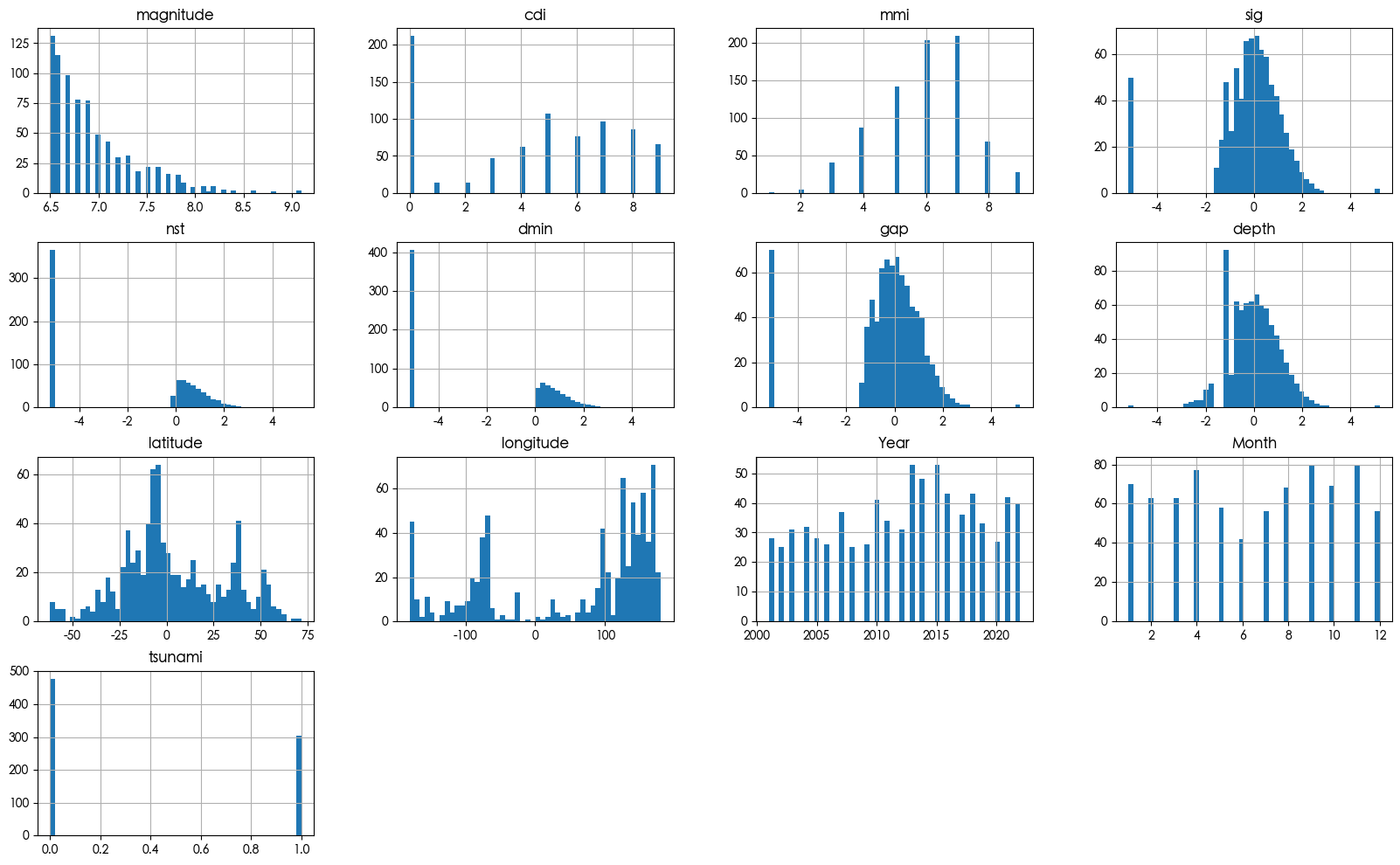
预处理 1 2 3 4 from sklearn.preprocessing import QuantileTransformer qt = QuantileTransformer(output_distribution='normal' , random_state=42) df [['nst' , 'dmin' , 'gap' , 'depth' , 'sig' ]] = qt.fit_transform(df [['nst' , 'dmin' , 'gap' , 'depth' , 'sig' ]])
1 2 df.hist(bins=50, figsize=(20,12)) plt.show()
方法1:SphericalRBF+LGBM 背景:为什么不能直接对经纬度做 RBF 如果你直接在纬度 (lat) 和经度 (lon) 上应用普通的 RBF 核:
$$
看似可行,但数学上是错误的,因为地球是一个球面,而 (lat, lon) 是球面坐标,并不满足欧几里得距离的几何意义。
对比:普通 RBF vs 球面 RBF
特征
普通 RBF on (Lat, Lon)
球面 RBF (Spherical RBF)
使用的距离
欧几里得距离(平面直线)
球面大圆距离(沿球面最短路径)
数学表达
$exp(-γ · ((Δlat)² + (Δlon)²))$
$exp(-γ · θ²)$,其中 $θ = arccos(u · u’)$
坐标空间
平面坐标系
单位球面(通过三维向量化)
近极点失真
严重失真(经度差在高纬度几乎没意义)
自动修正(以真实角距离计算)
经度 180° 跨越问题
错误:179°E 与 179°W 被认为相距 358°
正确:球面上仅相距 2°
适用范围
小区域、局部近似(如城市级)
全球范围(地球、天体等球面数据)
几何原理详解 假设两个点分别为:
点 A:纬度 $lat₁$,经度 $lon₁$
点 B:纬度 $lat₂$,经度 $lon₂$
普通 RBF 计算 $$
假设球面是平的。
在赤道附近还能勉强近似,但在两极或跨经度时会严重失真。
Spherical RBF 计算 先把每个点转换成球面单位向量:
$$
两个点的球面角距离为:
$$
于是 RBF 特征为:
$$
这意味着两点的“相似度”由球面上沿弧线的角度距离决定,而非平面直线距离。
在 SphericalRBF 类中如何实现
代码部分
含义
_to_unit()把 (lat, lon) → 单位球面坐标 (x, y, z)
fit()用 KMeans 在球面上找一组中心点
transform()计算每个样本到这些中心的球面角距离 θ,并用 $exp(-γ·θ²)$ 得到特征值
输出特征
每个样本对应一组“地理位置相似度”特征,可供机器学习模型使用
1 2 3 4 5 6 7 8 9 10 11 12 13 14 15 16 17 18 19 20 21 22 23 24 25 26 27 28 29 30 31 32 33 34 35 36 37 38 39 40 41 from sklearn.base import BaseEstimator, TransformerMixin from sklearn.cluster import KMeans import numpy as np class SphericalRBF(BaseEstimator, TransformerMixin): def __init__(self, n_clusters=5, gamma="auto" , random_state=None): self.n_clusters = n_clusters self.gamma = gamma self.random_state = random_state def _to_unit(self, lat, lon): lat, lon = np.radians(lat), np.radians(lon) x = np.cos(lat)*np.cos(lon) y = np.cos(lat)*np.sin(lon) z = np.sin(lat) return np.c_[x, y, z] def fit(self, X, y=None, sample_weight=None): X_array = X.values U = self._to_unit(X_array[:, 0], X_array[:, 1]) self.kmeans_ = KMeans( n_clusters=self.n_clusters, n_init="auto" , random_state=self.random_state ).fit(U, sample_weight=sample_weight) dot = U @ self.kmeans_.cluster_centers_.T ang = np.arccos(np.clip(dot, -1.0, 1.0)) med = np.median(ang[ang > 0]) if np.any(ang > 0) else 0.1 self.gamma_ = (1.0 / (2 * med ** 2)) if self.gamma == "auto" else float (self.gamma) return self def transform(self, X): X_array = X.values U = self._to_unit(X_array[:, 0], X_array[:, 1]) dot = U @ self.kmeans_.cluster_centers_.T ang = np.arccos(np.clip(dot, -1.0, 1.0)) return np.exp(-self.gamma_ * ang ** 2) def get_feature_names_out(self, names=None): return np.array([f"geo_cluster_{i}" for i in range(self.n_clusters)])
1 2 3 from sklearn.model_selection import train_test_split X_train, X_test, y_train, y_test = train_test_split(df.drop(columns=['tsunami' ]),df ['tsunami' ], test_size=0.2, stratify=df ['tsunami' ], random_state=42)
1 2 3 4 5 6 7 8 9 geo_sim = SphericalRBF(n_clusters=5, random_state=42) from sklearn.preprocessing import StandardScaler from sklearn.compose import ColumnTransformer preprocessor = ColumnTransformer([ ("geo" , geo_sim, ["latitude" , "longitude" ]), ("num" , StandardScaler(), ['magnitude' ,'cdi' ,'mmi' ,'sig' ,'nst' ,'dmin' ,'gap' ,'depth' ,'Year' ,'Month' ]) ])
1 2 3 4 5 6 7 8 9 10 11 12 13 14 15 from sklearn.pipeline import Pipeline from lightgbm import LGBMClassifier LGBM = Pipeline([ ('preprocessor' , preprocessor), ('model' , LGBMClassifier( objective='binary' , random_state=42, n_estimators=500, learning_rate=0.05, num_leaves=31, verbosity=-1 )) ])
1 2 3 4 5 6 7 8 9 10 11 from sklearn.model_selection import cross_val_score tree_clf = cross_val_score(LGBM, X=df.drop(columns=['tsunami' ]), y=df ['tsunami' ], scoring="accuracy" , cv=10) cv_scores = cross_val_score(LGBM, X=df.drop(columns=['tsunami' ]), y=df ['tsunami' ], scoring='accuracy' , cv=10) print (pd.Series(cv_scores).describe())
count 10.000000
1 2 3 4 5 6 7 LGBM.fit(X_train, y_train) train_acc = LGBM.score(X_train, y_train) test_acc = LGBM.score(X_test, y_test) print (f"Train Accuracy: {train_acc:.3f}" )print (f"Test Accuracy: {test_acc:.3f}" )
Train Accuracy: 1.000
方法2:三维球面坐标展开 1 2 3 4 5 df2 = df.copy() df2['x' ] = np.cos(df2['latitude' ]) * np.cos(df2['longitude' ]) df2['y' ] = np.cos(df2['latitude' ]) * np.sin(df2['longitude' ]) df2['z' ] = np.sin(df2['latitude' ])
1 2 3 4 5 6 7 8 9 10 11 12 13 14 15 16 17 18 19 20 21 22 23 24 25 26 27 28 from sklearn.model_selection import train_test_split X = df2.drop(columns=['tsunami' , 'latitude' , 'longitude' ]) y = df2['tsunami' ] X_train, X_test, y_train, y_test = train_test_split( X, y, test_size=0.2, stratify=y, random_state=42 ) LGBM2 = LGBMClassifier( random_state=42, n_estimators=500, learning_rate=0.05, num_leaves=31, verbosity=-1 ) scores = cross_val_score(LGBM2, X, y, cv=10, scoring='accuracy' ) print (scores.mean(), scores.std())LGBM2.fit(X_train, y_train) train_acc = LGBM2.score(X_train, y_train) print (f"Train Accuracy: {train_acc:.3f}" )test_acc = LGBM2.score(X_test, y_test) print (f"Test Accuracy: {test_acc:.3f}" )
0.7195715676728336 0.23385761172061434