Lifestyle_and_Health_Risk_Prediction_Synthetic_Dataset

数据来源

https://www.kaggle.com/datasets/miadul/lifestyle-and-health-risk-prediction

查看数据

import pandas as pd

df = pd.read_csv('Lifestyle_and_Health_Risk_Prediction_Synthetic_Dataset.csv')
df.head()

df.info()

<class ‘pandas.core.frame.DataFrame’>
RangeIndex: 5000 entries, 0 to 4999
Data columns (total 12 columns):

Column Non-Null Count Dtype

---

0 age 5000 non-null int64
1 weight 5000 non-null int64
2 height 5000 non-null int64
3 exercise 5000 non-null object
4 sleep 5000 non-null float64
5 sugar_intake 5000 non-null object
6 smoking 5000 non-null object
7 alcohol 5000 non-null object
8 married 5000 non-null object
9 profession 5000 non-null object
10 bmi 5000 non-null float64
11 health_risk 5000 non-null object
dtypes: float64(2), int64(3), object(7)
memory usage: 468.9+ KB

缺失值查看和处理

df.isnull().sum()

age 0
weight 0
height 0
exercise 0
sleep 0
sugar_intake 0
smoking 0
alcohol 0
married 0
profession 0
bmi 0
health_risk 0
dtype: int64

异常值查看与处理

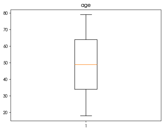
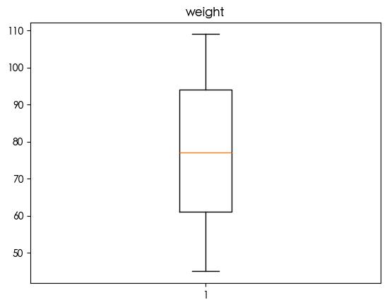
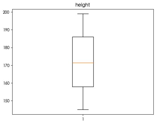
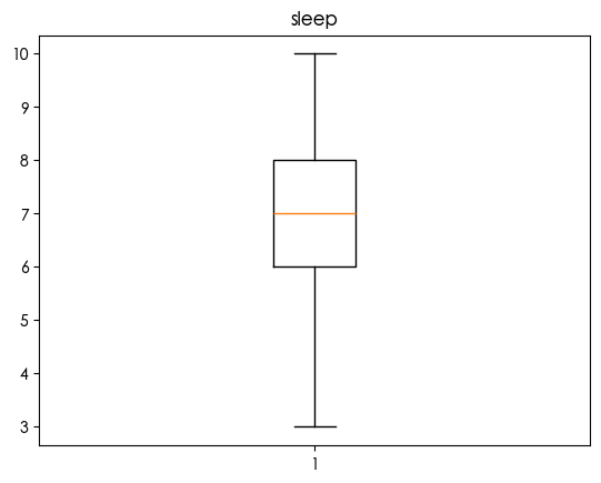
for column in df.select_dtypes(include=['number']).columns:
    plt.boxplot(df[column])
    plt.title(column)
    plt.show()

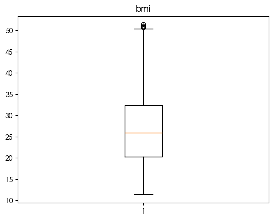
发现bmi存在异常值 鉴于bmi过高会导致健康风险 查看两者的关系

import seaborn as sns
import matplotlib.pyplot as plt

df_bmi_50 = df[df['bmi'] > 50]

sns.boxplot(x='health_risk', y='bmi', data=df_bmi_50)
plt.title('BMI与健康风险的关系')
plt.xlabel('健康风险')
plt.ylabel('BMI')
plt.show()

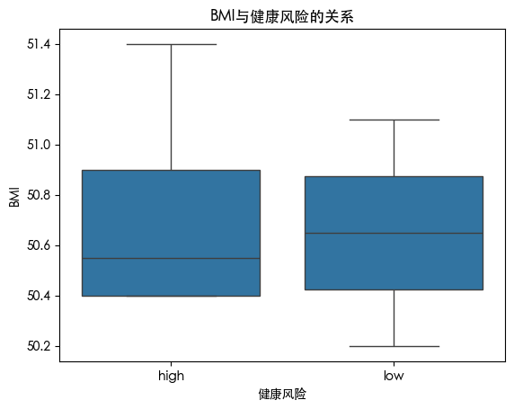
可以看到 健康风险较高的人群 其bmi最大值较高 但是在bmi>50的人群中 健康风险低的人群 bmi平均值要比健康风险高的人群高 这说明 衡量健康风险不仅仅看bmi 还要考虑其他因素

EDA

df['profession'].value_counts().plot(kind='bar')
plt.title('职业分布')
plt.show()

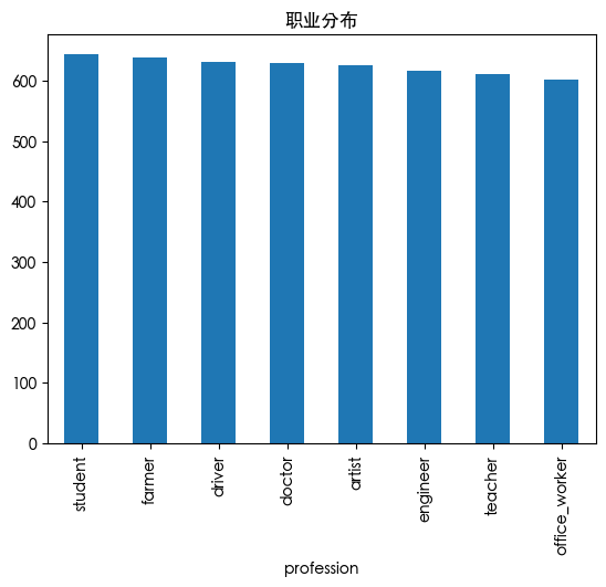
数据集中不同职业的数量分布是均衡的

age_groups = pd.cut(df['age'], bins=5)
ct = pd.crosstab(age_groups, df['health_risk'])


ct_pct = ct.div(ct.sum(axis=1), axis=0)
ct_pct.plot(
    kind='bar',
    stacked=True,
    figsize=(10, 6),
    color=['#f8f3d4', '#00b8a9']
    )
plt.title('健康风险与年龄分组的关系')
plt.xlabel('年龄分组')
plt.ylabel('百分比')
plt.xticks(rotation=45)
plt.legend(title='健康风险')
plt.tight_layout()
plt.show()

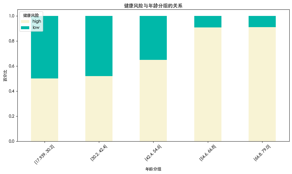
可以看到 随着年龄的增加 健康风险也在增加

import pandas as pd
import matplotlib.pyplot as plt

ct = pd.crosstab(df['exercise'], df['health_risk'])

exercise_order = ['none', 'low', 'medium', 'high']
ct = ct.reindex(exercise_order, fill_value=0)

ct_pct = ct.div(ct.sum(axis=1), axis=0) 
ct_pct.plot(
    kind='bar',
    stacked=True,
    figsize=(8, 6),
    color=['#f8f3d4', '#00b8a9']
)
plt.title('锻炼频率与健康风险的关系')
plt.xlabel('锻炼频率')
plt.ylabel('百分比')
plt.xticks(rotation=0)
plt.legend(title='健康风险')
plt.tight_layout()
plt.show()

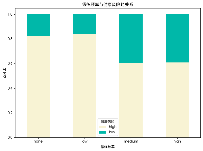
发现 锻炼频率高的人群 健康风险有明显的降低

sleep_groups = pd.cut(df['sleep'], bins=5)
ct = pd.crosstab(sleep_groups, df['health_risk'])

ct_pct = ct.div(ct.sum(axis=1), axis=0)
ct_pct.plot(
    kind='bar',
    stacked=True,
    figsize=(10, 6),
    color=['#f8f3d4', '#00b8a9']
    )
plt.title('健康风险与睡眠时长的关系')
plt.xlabel('睡眠分组')
plt.ylabel('百分比')
plt.xticks(rotation=45)
plt.legend(title='健康风险')
plt.tight_layout()
plt.show()

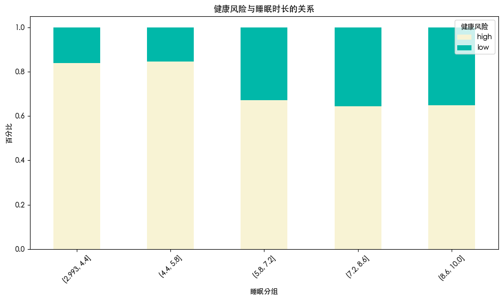
发现 睡眠时长长的人群 健康风险更低
更长的睡眠时间说明其睡眠质量更好 休息得更充分 这有助于提高健康水平

import pandas as pd
import matplotlib.pyplot as plt

ct = pd.crosstab(df['sugar_intake'], df['health_risk'])

sugar_order = ['low', 'medium', 'high']
ct = ct.reindex(sugar_order, fill_value=0)

ct_pct = ct.div(ct.sum(axis=1), axis=0) 
ct_pct.plot(
    kind='bar',
    stacked=True,
    figsize=(8, 6),
    color=['#f8f3d4', '#00b8a9']
)
plt.title('糖摄入量与健康风险的关系')
plt.xlabel('糖摄入量')
plt.ylabel('百分比')
plt.xticks(rotation=0)
plt.legend(title='健康风险')
plt.tight_layout()
plt.show()

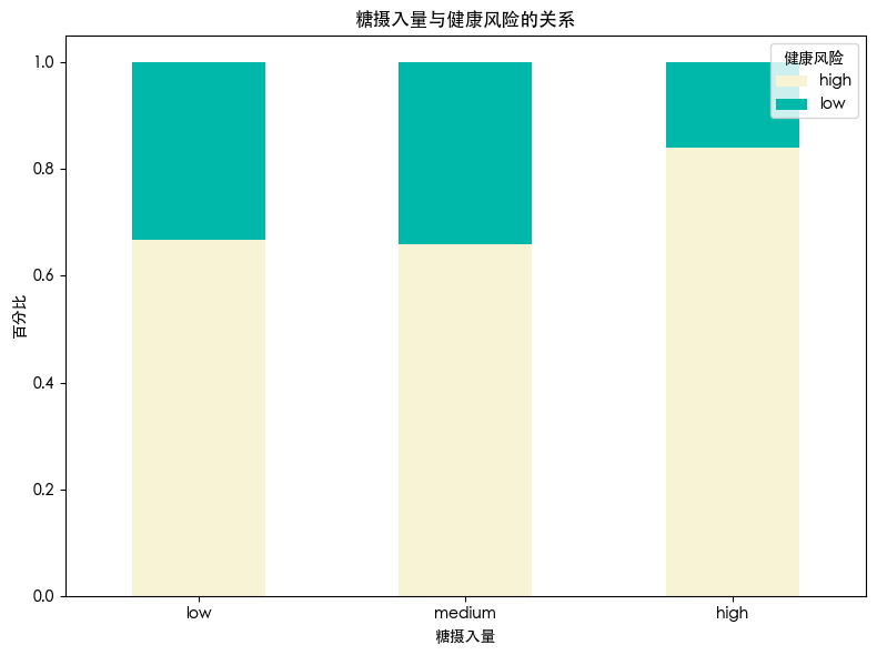
发现 糖摄入量高的人群 其健康风险更高 这可能是因为糖对身体的影响更大 会有患糖尿病的风险 导致健康风险增加

ct = pd.crosstab(df['smoking'], df['health_risk'])

smoking_order = ['yes', 'no']
ct = ct.reindex(smoking_order, fill_value=0)

ct_pct = ct.div(ct.sum(axis=1), axis=0) 
ct_pct.plot(
    kind='bar',
    stacked=True,
    figsize=(8, 6),
    color=['#f8f3d4', '#00b8a9']
)
plt.title('吸烟与健康风险的关系')
plt.xlabel('吸烟')
plt.ylabel('百分比')
plt.xticks(rotation=0)
plt.legend(title='健康风险')
plt.tight_layout()
plt.show()

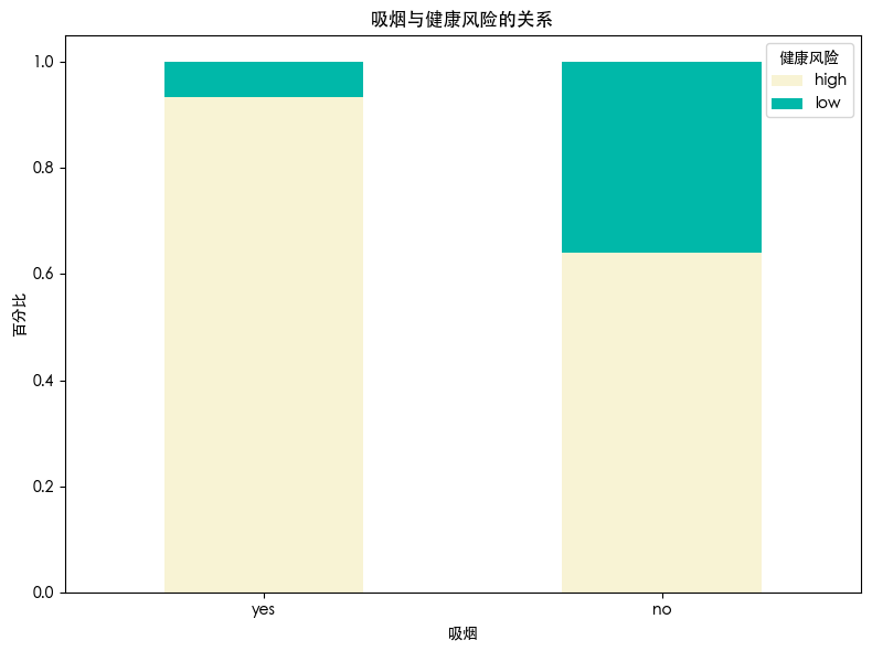
发现 不吸烟的人健康风险要比吸烟人的健康风险低
吸烟有患肺癌的风险

ct = pd.crosstab(df['alcohol'], df['health_risk'])

alcohol_order = ['yes', 'no']
ct = ct.reindex(alcohol_order, fill_value=0)

ct_pct = ct.div(ct.sum(axis=1), axis=0) 
ct_pct.plot(
    kind='bar',
    stacked=True,
    figsize=(8, 6),
    color=['#f8f3d4', '#00b8a9']
)
plt.title('饮酒与健康风险的关系')
plt.xlabel('饮酒')
plt.ylabel('百分比')
plt.xticks(rotation=0)
plt.legend(title='健康风险')
plt.tight_layout()
plt.show()

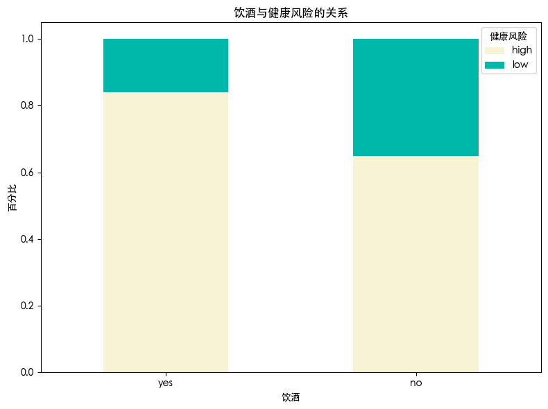
发现 不饮酒的人健康风险要比饮酒的人健康风险低
饮酒有患肝脏疾病的风险

ct = pd.crosstab(df['married'], df['health_risk'])

married_order = ['yes', 'no']
ct = ct.reindex(married_order, fill_value=0)

ct_pct = ct.div(ct.sum(axis=1), axis=0) 
ct_pct.plot(
    kind='bar',
    stacked=True,
    figsize=(8, 6),
    color=['#f8f3d4', '#00b8a9']
)
plt.title('婚姻状态与健康风险的关系')
plt.xlabel('婚姻状态')
plt.ylabel('百分比')
plt.xticks(rotation=0)
plt.legend(title='健康风险')
plt.tight_layout()
plt.show()

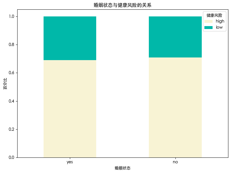
婚姻状况与健康风险的关系不明显 可以把这个特征删除

特征编码

对于exercise、sugar_intake、smoking、alcohol、married、health_risk
这些类别型特征是有明显大小关系的 因此使用标签编码保留其大小区别
对于profession由于特征中的值是无关的 并且特征中的唯一值只有8个 因此我们可以用独热编码

#标签编码

df['exercise'] = df['exercise'].map({'none': 0, 'low': 1, 'medium': 2, 'high': 3})
df['sugar_intake'] = df['sugar_intake'].map({'low': 0, 'medium': 1, 'high': 2})
df['smoking'] = df['smoking'].map({'yes': 1, 'no': 0})
df['alcohol'] = df['alcohol'].map({'yes': 1, 'no': 0})
df['married'] = df['married'].map({'yes': 1, 'no': 0})
df['health_risk'] = df['health_risk'].map({'low': 0, 'high': 1})

# 独热编码
df = pd.get_dummies(df, columns=['profession'], drop_first=True)

# 删除'married'列
df = df.drop(columns=['married'])

数据划分

from sklearn.model_selection import train_test_split

X = df.drop(columns=['health_risk'])
y = df['health_risk']

X_train, X_test, y_train, y_test = train_test_split(X, y, test_size=0.2, random_state=42)

模型选择

from sklearn.linear_model import LogisticRegression
from sklearn.ensemble import RandomForestClassifier
from sklearn.svm import SVC
from xgboost import XGBClassifier
from lightgbm import LGBMClassifier

model = {
    'logistic_regression': LogisticRegression(),
    'random_forest': RandomForestClassifier(),
    'svm': SVC(),
    'XGB': XGBClassifier(),
    'LGBM': LGBMClassifier()
}

from sklearn.metrics import accuracy_score, precision_score, recall_score, f1_score,classification_report,confusion_matrix
model_scores = pd.DataFrame(
    index=model.keys(),
    columns=[
        "accuracy",
        "precision",
        "recall",
        "f1_score",
        "cross_val_score"
    ]
)

for name, clf in model.items():
    clf.fit(X_train, y_train)
    print(f"{name}模型训练完成")
    y_pred = clf.predict(X_test)
    print(f"{name}模型测试结果")
    print(classification_report(y_test, y_pred))
    print(confusion_matrix(y_test, y_pred))
    print('----------------------------------------')
    model_scores.loc[name, "accuracy"] = accuracy_score(y_test, y_pred)
    model_scores.loc[name, "precision"] = precision_score(y_test, y_pred)
    model_scores.loc[name, "recall"] = recall_score(y_test, y_pred)
    model_scores.loc[name, "f1_score"] = f1_score(y_test, y_pred)

k折交叉验证

from sklearn.model_selection import cross_val_score

for name, clf in model.items():
    scores = cross_val_score(clf, X, y, cv=5)
    print(f"{name}模型的交叉验证得分: {scores.mean()}")
    model_scores.loc[name, "cross_val_score"] = scores.mean()

model_scores.head()

Model	Accuracy	Precision	Recall	F1_Score	Cross_Val_Score
logistic_regression	0.858	0.893056	0.908192	0.90056	0.8652
random_forest	0.99	0.992938	0.992938	0.992938	0.993
svm	0.804	0.829897	0.909605	0.867925	0.8076
XGB	0.995	0.997171	0.995763	0.996466	0.9966
LGBM	0.997	0.997179	0.998588	0.997883	0.9968

特征重要性

name = ['random_forest', 'XGB', 'LGBM']
for name in name:
    importances = pd.Series(model[name].feature_importances_, index=X_train.columns).sort_values(ascending=False)
    print(f"{name}模型特征重要性排序")
    print(importances)
    print('----------------------------------------')

• random_forest
• XGB
• LGBM

random_forest模型特征重要性排序
age 0.268261
bmi 0.182540
smoking 0.100002
exercise 0.094879
sleep 0.085877
weight 0.079399
sugar_intake 0.065287
alcohol 0.063469
height 0.038578
profession_teacher 0.003532
profession_doctor 0.003400
profession_student 0.003397
profession_engineer 0.003007
profession_driver 0.002944
profession_farmer 0.002875
profession_office_worker 0.002553
dtype: float64

XGB模型特征重要性排序
bmi 0.198563
smoking 0.173180
age 0.148690
alcohol 0.139040
exercise 0.122766
sugar_intake 0.114938
sleep 0.075064
profession_doctor 0.007731
profession_engineer 0.005987
profession_student 0.004006
profession_farmer 0.002454
profession_driver 0.002379
weight 0.002147
height 0.001987
profession_teacher 0.001068
profession_office_worker 0.000000
dtype: float32

LGBM模型特征重要性排序
sleep 614
sugar_intake 416
exercise 406
smoking 371
bmi 339
alcohol 337
age 298
height 99
weight 66
profession_doctor 14
profession_engineer 10
profession_farmer 10
profession_student 8
profession_teacher 7
profession_driver 5
profession_office_worker 0
dtype: int32