声明 本文代码均保存在https://github.com/super-213/business_data_analysis
导入库 1 2 3 4 5 6 7 8 9 import tushare as ts import numpy as np import pandas as pd import talib import matplotlib.pyplot as plt from sklearn.ensemble import RandomForestClassifier from sklearn.metrics import accuracy_score import warnings warnings.filterwarnings("ignore" )
1 2 3 4 5 6 7 8 9 10 11 12 13 14 15 16 17 18 19 20 21 22 23 24 df = ts.get_k_data('000002' ,start='2015-01-01' ,end='2019-12-31' )df = df.set_index('date' ) df ['close-open' ] = (df ['close' ] - df ['open' ])/df['open' ]df ['high-low' ] = (df ['high' ] - df ['low' ])/df['low' ]df ['pre_close' ] = df ['close' ].shift (1) df ['price_change' ] = df ['close' ]-df ['pre_close' ]df ['p_change' ] = (df ['close' ]-df ['pre_close' ])/df['pre_close' ]*100df ['MA5' ] = df ['close' ].rolling(5).mean()df ['MA10' ] = df ['close' ].rolling(10).mean()df.dropna(inplace=True) df ['RSI' ] = talib.RSI(df ['close' ], timeperiod=12) df ['MOM' ] = talib.MOM(df ['close' ], timeperiod=5) df ['EMA12' ] = talib.EMA(df ['close' ], timeperiod=12) df ['EMA26' ] = talib.EMA(df ['close' ], timeperiod=26) df ['MACD' ], df ['MACDsignal' ], df ['MACDhist' ] = talib.MACD(df ['close' ], fastperiod=12, slowperiod=26, signalperiod=9) df.dropna(inplace=True)
库太老了 我使用其他数据获取库
akshare
pip install akshare
查看数据 1 2 3 4 5 import akshare as ak df = ak.stock_zh_a_hist(symbol="000002" , period="daily" , start_date="20150101" , end_date="20191231" , adjust="" )df = df.set_index('日期' )df.head()
日期
股票代码
开盘
收盘
最高
最低
成交量
成交额
振幅
涨跌幅
涨跌额
换手率
2015-01-05
000002
14.39
14.91
15.29
14.22
6560836
9.700712e+09
7.70
7.27
1.01
6.76
2015-01-06
000002
14.60
14.36
14.99
14.05
3346347
4.839616e+09
6.30
-3.69
-0.55
3.45
2015-01-07
000002
14.26
14.23
14.50
14.00
2642051
3.772151e+09
3.48
-0.91
-0.13
2.72
2015-01-08
000002
14.32
13.59
14.37
13.46
2639394
3.629554e+09
6.39
-4.50
-0.64
2.72
2015-01-09
000002
13.54
13.45
14.22
13.29
3294584
4.521978e+09
6.84
-1.03
-0.14
3.39
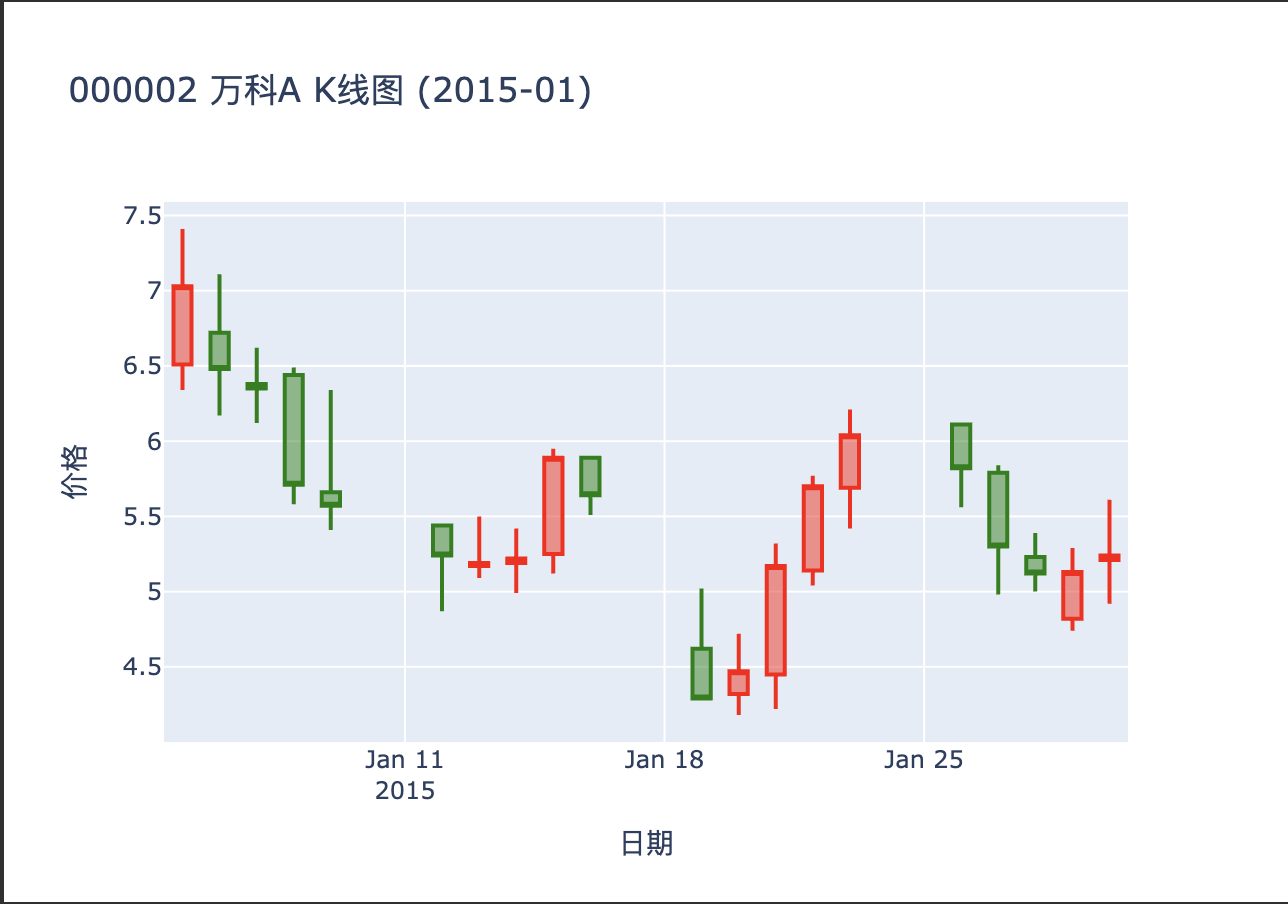
画k线图 针对股票市场 我们肯定要查看其k线图
1 2 3 4 5 6 7 8 9 10 11 12 13 14 15 16 17 18 19 20 21 22 import plotly.graph_objects as go data = df.loc["2015-01-01" :"2015-01-31" ] fig = go.Figure(data=[go.Candlestick( x=data.index, open=data["Open" ], high=data["High" ], low=data["Low" ], close=data["Close" ], increasing_line_color="red" , decreasing_line_color="green" )]) fig.update_layout( title="000002 万科A K线图 (2015-01)" , xaxis_title="日期" , yaxis_title="价格" , xaxis_rangeslider_visible=False ) fig.show()
随机森林 1 2 3 4 5 6 7 8 9 10 11 12 13 14 15 16 17 18 19 20 21 22 23 24 import pandas as pd from sklearn.model_selection import train_test_split from sklearn.ensemble import RandomForestClassifier from sklearn.metrics import classification_report, accuracy_score df = ak.stock_zh_a_hist(symbol="000002" , period="daily" , start_date="20150101" , end_date="20150131" , adjust="qfq" )df ["label" ] = (df ["收盘" ].shift (-1) > df ["收盘" ]).astype(int) X = df [["开盘" , "最高" , "最低" , "收盘" , "成交量" , "成交额" , "振幅" , "涨跌幅" , "换手率" ]] y = df ["label" ] X = X[:-1] y = y[:-1] X_train, X_test, y_train, y_test = train_test_split(X, y, test_size=0.2, shuffle=False) rf = RandomForestClassifier(n_estimators=200, random_state=42) rf.fit(X_train, y_train) y_pred = rf.predict(X_test) print ("准确率:" , accuracy_score(y_test, y_pred))print (classification_report(y_test, y_pred))
准确率: 1.0
类别
Precision
Recall
F1-Score
Support
0
1.00
1.00
1.00
2
1
1.00
1.00
1.00
2
accuracy 1.00 4
macro avg 1.00
1.00
1.00
4
weighted avg 1.00
1.00
1.00
4
1
2
3
feature_importances = pd.Series(rf.feature_importances_, index=X.columns) feature_importances = feature_importances.sort_values(ascending=False) print (feature_importances)
特征
重要性
开盘
0.3772
最高
0.2516
最低
0.1511
收盘
0.1213
涨跌幅
0.0444
振幅
0.0196
成交量
0.0173
换手率
0.0095
成交额
0.0081
决策树 1 2 3 4 5 6 7 8 from sklearn.tree import DecisionTreeClassifier dtc = DecisionTreeClassifier(random_state=42) dtc.fit(X_train, y_train) y_pred = dtc.predict(X_test) from sklearn.metrics import classification_report, confusion_matrix print (confusion_matrix(y_test, y_pred))print (classification_report(y_test, y_pred))
类别
Precision
Recall
F1-Score
Support
0
0.67
1.00
0.80
2
1
1.00
0.50
0.67
2
accuracy 0.75 4
macro avg 0.83
0.75
0.73
4
weighted avg 0.83
0.75
0.73
4
1 2 3 4 5 6 from sklearn.model_selection import cross_val_score scores = cross_val_score(dtc, X_train, y_train, cv=5, scoring='accuracy' ) print ("各折准确率:" , scores)print ("平均准确率:%.4f (+/- %.4f)" % (scores.mean(), scores.std() * 2))
各折准确率: [1. 1. 0.66666667 0.66666667 1. ]
决策树结果分析 发现决策树效果并没有随机森林那么好 这是因为随机森林是一种集成算法 是由多个决策树集成的 其结果是由多个决策树共同打分的 因此随机森林在处高维数据时会比决策树要好
GBDT 1 2 3 4 5 6 7 8 from sklearn.ensemble import GradientBoostingClassifier GBDT = GradientBoostingClassifier(random_state=42) GBDT.fit(X_train, y_train) y_pred = GBDT.predict(X_test) print (confusion_matrix(y_test, y_pred))print (classification_report(y_test, y_pred))
类别
Precision
Recall
F1-Score
Support
0
0.67
1.00
0.80
2
1
1.00
0.50
0.67
2
accuracy 0.75 4
macro avg 0.83
0.75
0.73
4
weighted avg 0.83
0.75
0.73
4
1 2 3 4 5 6 from sklearn.model_selection import cross_val_score scores = cross_val_score(GBDT, X_train, y_train, cv=5, scoring='accuracy' ) print ("各折准确率:" , scores)print ("平均准确率:%.4f (+/- %.4f)" % (scores.mean(), scores.std() * 2))
各折准确率: [1. 1. 0.66666667 0.66666667 1. ]
GBDT结果分析 发现GBDT的结果没随机森林要好 这是因为GBDT对参数敏感 需要进行调参 使用网格优化
1 2 3 4 5 6 7 8 9 10 11 12 13 14 15 16 17 18 19 20 21 from sklearn.model_selection import GridSearchCV param_grid = { 'n_estimators' : [100, 200, 500], 'learning_rate' : [0.1, 0.05, 0.01], 'max_depth' : [3, 5, 7], 'min_samples_split' : [2, 5, 10], 'min_samples_leaf' : [1, 2, 4] } grid = GridSearchCV( GradientBoostingClassifier(random_state=42), param_grid, cv=5, scoring='f1_macro' , n_jobs=-1 ) grid.fit(X_train, y_train) print ("Best Params:" , grid.best_params_)print ("Best Score:" , grid.best_score_)
Best Params: {‘learning_rate’: 0.1, ‘max_depth’: 3, ‘min_samples_leaf’: 1, ‘min_samples_split’: 2, ‘n_estimators’: 100}
朴素贝叶斯 1 2 3 4 5 6 7 8 9 10 11 12 13 14 from sklearn.naive_bayes import GaussianNB nb = GaussianNB() nb.fit(X_train, y_train) y_pred_nb = nb.predict(X_test) y_pred_proba = nb.predict_proba(X_test)[:, 1] print ("混淆矩阵:" )print (confusion_matrix(y_test, y_pred_nb))print ("\n分类报告:" )print (classification_report(y_test, y_pred_nb))print ("\n前5个样本的离职概率:" , y_pred_proba[:5])
1
2
3
4
5
6
from sklearn.model_selection import cross_val_score scores = cross_val_score(nb, X_train, y_train, cv=5, scoring='accuracy' ) print ("各折准确率:" , scores)print ("平均准确率:%.4f (+/- %.4f)" % (scores.mean(), scores.std() * 2))
贝叶斯结果分析 可以看到 贝叶斯的结果非常不好 这是因为 贝叶斯模型是假设特征之间是相互独立的 而在股票市场中 特征之间往往是存在相关性的 因此贝叶斯模型的效果是要比其他模型差的
我们还可以画出特征之间的热力图
1 2 3 4 5 import seaborn as sns correlation_matrix = pd.concat([X_train, y_train], axis=1).corr() sns.heatmap(correlation_matrix, annot=True, cmap='coolwarm' ) plt.show()
可以看到 像开盘与最高 开盘与最低等之间呈现高相关性
LDA 1 2 3 4 5 6 7 8 9 10 11 from sklearn.discriminant_analysis import LinearDiscriminantAnalysis LDA = LinearDiscriminantAnalysis() LDA.fit(X_train, y_train) y_pred_lda = LDA.predict(X_test) y_pred_proba_lda = LDA.predict_proba(X_test)[:, 1] print ("混淆矩阵:" )print (confusion_matrix(y_test, y_pred_lda))print ("\n分类报告:" )print (classification_report(y_test, y_pred_lda))
类别
Precision
Recall
F1-Score
Support
0
1.00
1.00
1.00
2
1
1.00
1.00
1.00
2
accuracy 1.00 4
macro avg 1.00
1.00
1.00
4
weighted avg 1.00
1.00
1.00
4
1
2
3
4
5
6
from sklearn.model_selection import cross_val_score scores = cross_val_score(LDA, X_train, y_train, cv=5, scoring='accuracy' ) print ("各折准确率:" , scores)print ("平均准确率:%.4f (+/- %.4f)" % (scores.mean(), scores.std() * 2))
各折准确率: [0.66666667 0.66666667 0.66666667 0.66666667 0.33333333]
LDA结果分析 我们看到 LDA的分类报告非常好 但是进行k折交叉验证的时候没那么好
1
2
3
4
5
6
from sklearn.model_selection import TimeSeriesSplit, cross_val_score tscv = TimeSeriesSplit(n_splits=5) scores = cross_val_score(LDA, X_train, y_train, cv=tscv, scoring='accuracy' ) print ("各折准确率:" , scores)print ("平均准确率:%.4f (+/- %.4f)" % (scores.mean(), scores.std() * 2))
各折准确率: [0.5 0.5 0.5 0.5 0.5]
LDA 假设特征服从高斯分布 且协方差矩阵相同 但股票特征往往不满足