商业数据分析--信用卡精准营销模型

声明

本文代码均保存在
https://github.com/super-213/business_data_analysis
有需要的可以自行下载

查看数据

df =pd.read_excel('信用卡精准营销模型.xlsx')
df.head()

年龄	月收入（元）	月消费（元）	性别	月消费/月收入	响应
30	7275	6062	0	0.833265	1
25	17739	13648	0	0.769378	1
29	25736	14311	0	0.556069	1
23	14162	7596	0	0.536365	1
27	15563	12849	0	0.825612	1

缺失值处理

df.isnull().sum()

字段	缺失值数量
年龄	0
月收入（元）	0
月消费（元）	0
性别	0
月消费/月收入	0
响应	0

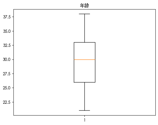
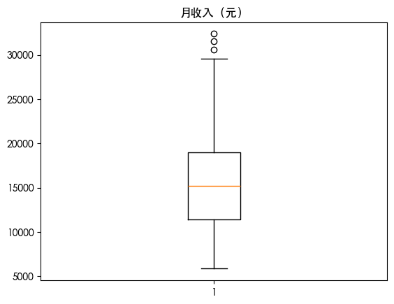
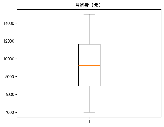
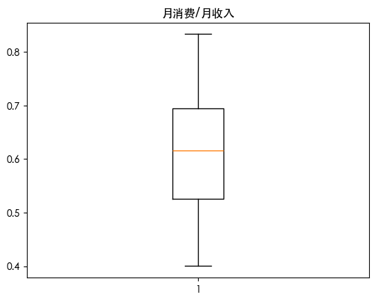
异常值处理

for col in df.columns:
    if df[col].dtype in ['int64', 'float64']:
        plt.boxplot(df[col])
        plt.title(col)
        plt.show()
    else:
        df[col].value_counts().plot(kind='bar')
        plt.title(col)
        plt.show()

数据划分

from sklearn.model_selection import train_test_split

X = df.drop(['响应'], axis=1)
y = df['响应']

X_train, X_test, y_train, y_test = train_test_split(X, y, test_size=0.2, random_state=42)

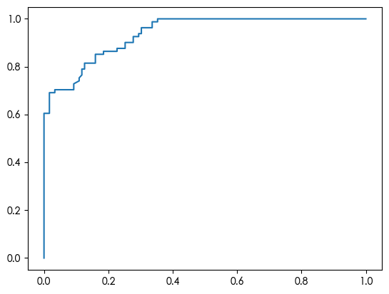
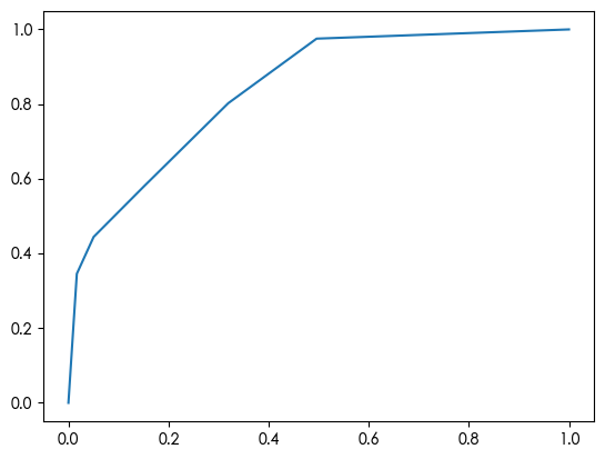
AdaBoost

from sklearn.ensemble import AdaBoostClassifier
adab = AdaBoostClassifier(random_state=123)
adab.fit(X_train, y_train)
y_pred = adab.predict(X_test)
from sklearn.metrics import accuracy_score

accuracy = accuracy_score(y_test, y_pred)
print("Accuracy:", accuracy)
from sklearn.metrics import confusion_matrix

cm = confusion_matrix(y_test, y_pred)
print("Confusion Matrix:\n", confusion_matrix)
from sklearn.metrics import classification_report
print(classification_report(y_test, y_pred))

from sklearn.metrics import roc_curve

y_pred_proba = adab.predict_proba(X_test)
fpr, tpr, thres = roc_curve(y_test.values, y_pred_proba[:,1])
import matplotlib.pyplot as plt
plt.plot(fpr, tpr)
plt.show()

Accuracy: 0.83

实际 \ 预测	0	1
0	—	—
1	—	—

类别	Precision	Recall	F1-Score	Support
0	0.83	0.89	0.86	119
1	0.82	0.74	0.78	81
accuracy			0.83	200
macro avg	0.83	0.82	0.82	200
weighted avg	0.83	0.83	0.83	200

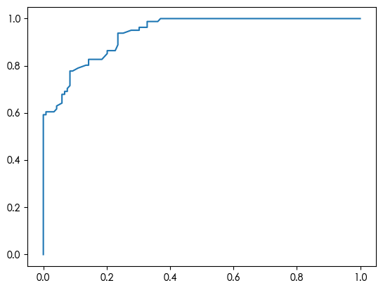
随机森林

from sklearn.ensemble import RandomForestClassifier

rm = RandomForestClassifier(random_state=42)
rm.fit(X_train, y_train)
y_pred = rm.predict(X_test)
print(confusion_matrix(y_test, y_pred))
print(classification_report(y_test, y_pred))

feature_importance = pd.DataFrame({
    "feature": X_train.columns,
    "importance": rm.feature_importances_
}).sort_values(by="importance", ascending=False)
print(feature_importance)

from sklearn.metrics import roc_curve

y_pred_proba = rm.predict_proba(X_test)
fpr, tpr, thres = roc_curve(y_test.values, y_pred_proba[:,1])
import matplotlib.pyplot as plt
plt.plot(fpr, tpr)
plt.show()

Accuracy: 0.83

实际 \ 预测	0	1
0	109	10
1	23	58

类别	Precision	Recall	F1-Score	Support
0	0.83	0.92	0.87	119
1	0.85	0.72	0.78	81
accuracy			0.83	200
macro avg	0.84	0.82	0.82	200
weighted avg	0.84	0.83	0.83	200

feature	importance
月消费/月收入	0.360143
月消费（元）	0.264454
年龄	0.206565
月收入（元）	0.143241
性别	0.025597

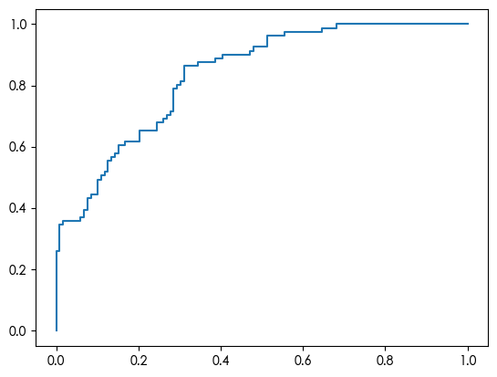
XGBoost

from xgboost import XGBClassifier

xgb = XGBClassifier()
xgb.fit(X_train, y_train)
y_pred_xgb = xgb.predict(X_test)
print(classification_report(y_test, y_pred_xgb))

feature_importance = pd.DataFrame({
    "feature": X_train.columns,
    "importance": xgb.feature_importances_
}).sort_values(by="importance", ascending=False)
print(feature_importance)

from sklearn.metrics import roc_curve

y_pred_proba = xgb.predict_proba(X_test)
fpr, tpr, thres = roc_curve(y_test.values, y_pred_proba[:,1])
import matplotlib.pyplot as plt
plt.plot(fpr, tpr)
plt.show()

类别	Precision	Recall	F1-Score	Support
0	0.85	0.90	0.87	119
1	0.84	0.77	0.80	81
accuracy			0.84	200
macro avg	0.84	0.83	0.84	200
weighted avg	0.84	0.84	0.84	200

feature	importance
月消费/月收入	0.284714
年龄	0.270551
月消费（元）	0.214029
性别	0.140819
月收入（元）	0.089888

SVM

from sklearn.svm import SVC

svc = SVC(probability=True)
svc.fit(X_train, y_train)
y_pred_svc = svc.predict(X_test)

print(classification_report(y_test, y_pred_svc))

from sklearn.metrics import roc_curve

y_pred_proba = svc.predict_proba(X_test)
fpr, tpr, thres = roc_curve(y_test.values, y_pred_proba[:,1])
import matplotlib.pyplot as plt
plt.plot(fpr, tpr)
plt.show()

类别	Precision	Recall	F1-Score	Support
0	0.72	0.88	0.80	119
1	0.75	0.51	0.60	81
accuracy			0.73	200
macro avg	0.73	0.69	0.70	200
weighted avg	0.73	0.73	0.72	200

KNN

from sklearn.neighbors import KNeighborsClassifier

knn = KNeighborsClassifier(n_neighbors=5)
knn.fit(X_train, y_train)
y_pred_knn = knn.predict(X_test)

print(classification_report(y_test, y_pred_knn))

y_pred_proba = knn.predict_proba(X_test)
fpr, tpr, thres = roc_curve(y_test.values, y_pred_proba[:,1])
import matplotlib.pyplot as plt
plt.plot(fpr, tpr)
plt.show()

类别	Precision	Recall	F1-Score	Support
0	0.75	0.85	0.80	119
1	0.72	0.58	0.64	81
accuracy			0.74	200
macro avg	0.74	0.71	0.72	200
weighted avg	0.74	0.74	0.73	200

模型横向比较

分类报告比较

模型	Accuracy	Precision (正类)	Recall (正类)	F1-Score (正类)	特点/说明
AdaBoost	0.83	0.82	0.74	0.78	强调难分类样本的迭代加权，适合弱分类器组合；可能对噪声敏感。
随机森林	0.83	0.85	0.72	0.78	多棵决策树投票，抗过拟合能力强，对特征相关性不敏感；正负类召回存在差异。
XGBoost	0.84	0.84	0.77	0.80	梯度提升树，学习能力强、对非线性关系拟合优秀；特征重要性分布较合理。
SVM	0.73	0.75	0.51	0.60	对高维线性可分表现好，非线性需核函数；对不平衡数据敏感，召回率偏低。
KNN	0.74	0.72	0.58	0.64	基于距离度量，易受噪声和特征尺度影响；正类召回明显低于树模型。

混淆矩阵对比

模型	TP	FN	FP	TN
AdaBoost	58	23	10	109
随机森林	58	23	10	109
XGBoost	62	19	14	105
SVM	41	40	18	101
KNN	47	34	18	101

说明：

• 树模型（AdaBoost、随机森林、XGBoost）对正类和负类的预测都相对均衡，XGBoost略优。
• SVM 和 KNN 正类召回较低，导致 F1-Score 较低。
• XGBoost 正类召回率比随机森林和 AdaBoost 更高，因此 F1-Score 也略高。

特征重要性对比

特征	AdaBoost	随机森林	XGBoost
月消费/月收入	0.36	0.36	0.28
月消费（元）	0.26	0.26	0.21
年龄	0.21	0.21	0.27
月收入（元）	0.14	0.14	0.09
性别	0.03	0.03	0.14

说明：

• XGBoost 更看重年龄和性别的作用，而 AdaBoost 和随机森林更侧重消费特征。
• 特征权重差异会导致不同模型在正类和负类上的表现略有不同。

模型结果差异原因分析

1. 算法机制不同：

   • 树模型（随机森林、XGBoost、AdaBoost）通过划分特征空间拟合非线性关系，对类别不平衡具有一定容错。
   • SVM 偏向最大化间隔，对于非线性和不平衡数据，召回率下降。
   • KNN 依赖邻近样本，易受噪声和数据分布影响，导致正类召回低。

2. 正负类不平衡：

   • 树模型可通过样本加权（AdaBoost）或集成投票（随机森林、XGBoost）缓解。
   • SVM 和 KNN 对不平衡敏感，正类容易被误判。

3. 特征处理和重要性：

   • 不同模型对特征敏感性不同，例如 SVM 对尺度敏感，KNN 对距离敏感，而树模型不敏感。
   • 特征重要性分布不同会直接影响模型预测偏向，尤其是在正负类分布不均时。

4. 模型调参与复杂度：

   • XGBoost 提供更多正则化和优化手段，因此整体 F1 更高。
   • AdaBoost 使用简单弱分类器叠加，效果略低于 XGBoost。
   • KNN、SVM 调参未充分时容易欠拟合或偏向负类。

总结

• XGBoost 综合表现最佳，F1-Score、Accuracy 较高，正类召回也不错。
• 随机森林、AdaBoost 次之，均衡性良好。
• SVM、KNN 表现较差，主要受类别不平衡和特征尺度影响，正类召回明显低。
• 模型选择需考虑任务需求：若更关注正类召回，XGBoost 和随机森林更适合；若对整体准确率要求高，AdaBoost 也可考虑。