商业数据分析--客户信息及违约表现

声明

本文代码均保存在
https://github.com/super-213/business_data_analysis
有需要的可以自行下载

查看数据

df = pd.read_excel('客户信息及违约表现.xlsx')
df.head()

收入	年龄	性别	历史授信额度	历史违约次数	是否违约
462087	26	1	0	1	1
362324	32	0	13583	0	1
332011	52	1	0	1	1
252895	39	0	0	1	1
352355	50	1	0	0	1

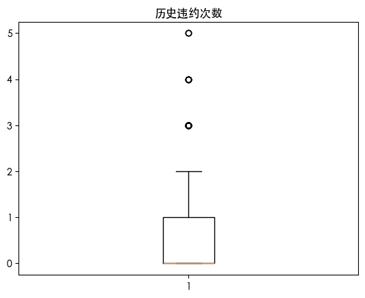
缺失值处理

df.isnull().sum()

异常值处理

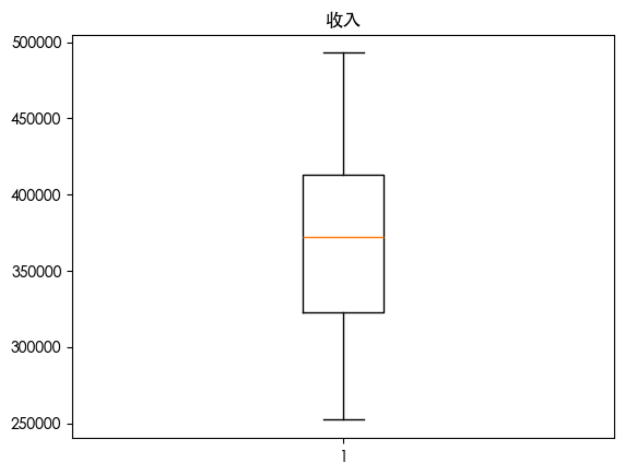
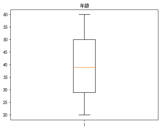
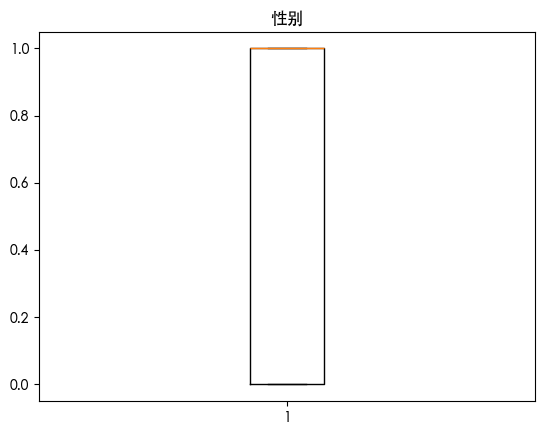
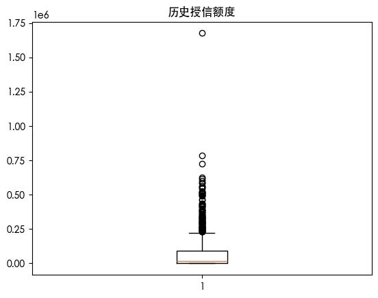
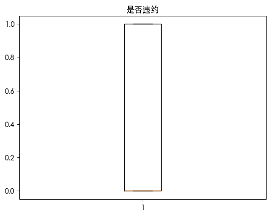
for col in df.columns:
    plt.boxplot(df[col])
    plt.title(col)
    plt.show()

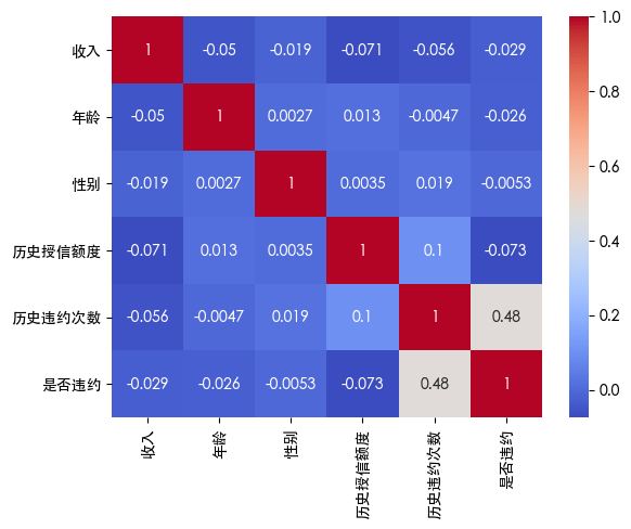
发现两个特征存在异常值 使用热力图查看特征之间的关系

import seaborn as sns

sns.heatmap(df.corr(), annot=True, cmap='coolwarm')
plt.show()

看到 历史违约次数和是否违约相关性很大 并且历史违约次数存在异常值 因此新增此特征的异常值特征列

col = '历史违约次数'

Q1 = df[col].quantile(0.25)
Q3 = df[col].quantile(0.75)
IQR = Q3 - Q1

lower_bound = Q1 - 1.5 * IQR
upper_bound = Q3 + 1.5 * IQR

df[f'{col}_is_outlier'] = ((df[col] < lower_bound) | (df[col] > upper_bound)).astype(int)

df = df.drop(columns=['历史授信额度'])

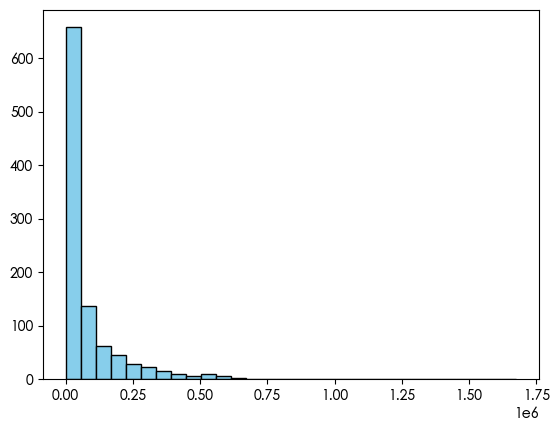
继续查看另一个异常值的特征分布

plt.hist(df['历史授信额度'], bins=30, color='skyblue', edgecolor='black')
plt.show()

可以看到 数据是右偏的 并且是长尾分布 对于此数据 使用对数变换

import numpy as np
col = '历史授信额度'
df[f'{col}_log'] = np.log1p(df[col])

数据划分

X = df.drop(columns=['是否违约'])
y = df['是否违约']

from sklearn.model_selection import train_test_split
X_train, X_test, y_train, y_test = train_test_split(X, y, test_size=0.2, random_state=42)

XGBoost

from xgboost import XGBClassifier

xgb = XGBClassifier(
    n_estimators=100,
    learning_rate=0.1,
    max_depth=5,
    subsample=0.8,
    colsample_bytree=0.8,
    random_state=42
)
xgb.fit(X_train, y_train)
y_pred = xgb.predict(X_test)

from sklearn.metrics import classification_report, confusion_matrix
print(confusion_matrix(y_test, y_pred))
print(classification_report(y_test, y_pred))

实际 \ 预测	0	1
0	110	9
1	29	52

类别	Precision	Recall	F1-Score	Support
0	0.79	0.92	0.85	119
1	0.85	0.64	0.73	81
accuracy			0.81	200
macro avg	0.82	0.78	0.79	200
weighted avg	0.82	0.81	0.80	200

LGBM

from lightgbm import LGBMClassifier

lgbm = LGBMClassifier(
    n_estimators=100,
    learning_rate=0.1,
    max_depth=5,
    subsample=0.8,
    colsample_bytree=0.8,
    random_state=42
)
lgbm.fit(X_train, y_train)
y_pred = lgbm.predict(X_test)

from sklearn.metrics import classification_report, confusion_matrix
print(confusion_matrix(y_test, y_pred))
print(classification_report(y_test, y_pred))

实际 \ 预测	0	1
0	113	6
1	29	52

类别	Precision	Recall	F1-Score	Support
0	0.80	0.95	0.87	119
1	0.90	0.64	0.75	81
accuracy			0.82	200
macro avg	0.85	0.80	0.81	200
weighted avg	0.84	0.82	0.82	200

随机森林

from sklearn.ensemble import RandomForestClassifier

rm = RandomForestClassifier(
    n_estimators=100,
    max_depth=5,
    random_state=42
)
rm.fit(X_train, y_train)
y_pred = rm.predict(X_test)

from sklearn.metrics import classification_report, confusion_matrix
print(confusion_matrix(y_test, y_pred))
print(classification_report(y_test, y_pred))

实际 \ 预测	0	1
0	117	2
1	29	52

类别	Precision	Recall	F1-Score	Support
0	0.80	0.98	0.88	119
1	0.96	0.64	0.77	81
accuracy			0.84	200
macro avg	0.88	0.81	0.83	200
weighted avg	0.87	0.84	0.84	200

贝叶斯

from sklearn.naive_bayes import GaussianNB

nb = GaussianNB()
nb.fit(X_train, y_train)
y_pred = nb.predict(X_test)

from sklearn.metrics import classification_report, confusion_matrix
print(confusion_matrix(y_test, y_pred))
print(classification_report(y_test, y_pred))

实际 \ 预测	0	1
0	111	8
1	43	38

类别	Precision	Recall	F1-Score	Support
0	0.72	0.93	0.81	119
1	0.83	0.47	0.60	81
accuracy			0.74	200
macro avg	0.77	0.70	0.71	200
weighted avg	0.76	0.74	0.73	200

逻辑回归

from sklearn.linear_model import LogisticRegression

lr = LogisticRegression()
lr.fit(X_train, y_train)
y_pred = lr.predict(X_test)

from sklearn.metrics import classification_report, confusion_matrix
print(confusion_matrix(y_test, y_pred))
print(classification_report(y_test, y_pred))

实际 \ 预测	0	1
0	88	31
1	60	21

类别	Precision	Recall	F1-Score	Support
0	0.59	0.74	0.66	119
1	0.40	0.26	0.32	81
accuracy			0.55	200
macro avg	0.50	0.50	0.49	200
weighted avg	0.52	0.55	0.52	200

模型横向对比

XGBoost

• 整体表现： Accuracy = 0.81
• 优点：
  • Precision 对 1 类 较高 (0.85)，但 Recall 偏低 (0.64)
  • 说明它比较谨慎 预测为违约时大多是真的（低假阳性）但漏掉了不少实际违约（高假阴性）
  • 适合在误判正常人为违约成本高的场景

LightGBM

• 整体表现： Accuracy = 0.82（略高于 XGB）
• 优点：
  • 对类别 1 的 Precision 更高 (0.90) Recall 同样偏低 (0.64)
  • 预测结果更保守 对 1 的识别严格 但仍漏掉一部分违约客户
  • 对比 XGBoost：性能非常接近，但 LightGBM 对类别 0 的 Recall 更高 对正常客户的识别更稳

随机森林

• 整体表现： Accuracy = 0.84
• 优点：
  • 类别 0 的 Recall 极高 几乎不会把正常客户错判为违约
  • 类别 1 的 Precision 很高 (0.96)，但 Recall 仍然只有 0.64 但还是漏掉部分
• 特点：
  • Bagging 思路让它在这类低维表格数据上表现最稳健。
  • 如果更在意总体准确率和稳健性，随机森林是首选。

朴素贝叶斯

• 整体表现： Accuracy = 0.74
• 优点： 对类别 0 Recall 较高
• 缺点： 类别 1 Recall 低 几乎一半违约客户都漏掉。
• 原因：
  • 假设特征独立，这在客户数据里往往不成立 会导致性能下降

逻辑回归

• 整体表现： Accuracy = 0.55
• 缺点：
  • 类别 1 的 Recall 极低 大部分违约客户被判成了正常
  • 说明数据中的关系并不是线性可分的 逻辑回归模型过于简单
• 适用场景：
  • 在数据高度线性且变量少时可用 但在这个复杂数据集上严重欠拟合

总结

模型	Accuracy	类别 1 (违约) Recall	特点
随机森林	0.84	0.64	最优表现，稳健，几乎不误判正常客户
LightGBM	0.82	0.64	高效，Precision 高，Recall 偏低
XGBoost	0.81	0.64	与 LGBM 接近，偏保守
朴素贝叶斯	0.74	0.47	偏弱，假设不符合实际
逻辑回归	0.55	0.26	严重欠拟合，不适合此任务

结论：

• 整体上 树模型（RF、XGB、LGBM）表现远优于线性模型（LR）和简单概率模型（NB）
• 随机森林在这里是最佳选择，因为它在准确率和稳定性上均优 并且对违约的准确率特别高
• 但三种树模型都有一个共性：违约 Recall 偏低（都在 0.64 左右） 意味着有不少违约客户没被识别出来