商业数据分析--客户价值数据表

声明

本文代码均保存在
https://github.com/super-213/business_data_analysis
有需要的可以自行下载

查看数据

我们首先查看数据

df = pd.read_excel('客户价值数据表.xlsx')

df.head()

	客户价值	历史贷款金额	贷款次数	学历	月收入	性别
0	1150	6488	2	2	9567	1
1	1157	5194	4	2	10767	0
2	1163	7066	3	2	9317	0
3	983	3550	3	2	10517	0
4	1205	7847	3	3	11267	1

在这个数据中 客户价值是我们要预测的目标

df.isnull().sum()

客户价值	0
历史贷款金额	0
贷款次数	0
学历	0
月收入	0
性别	0

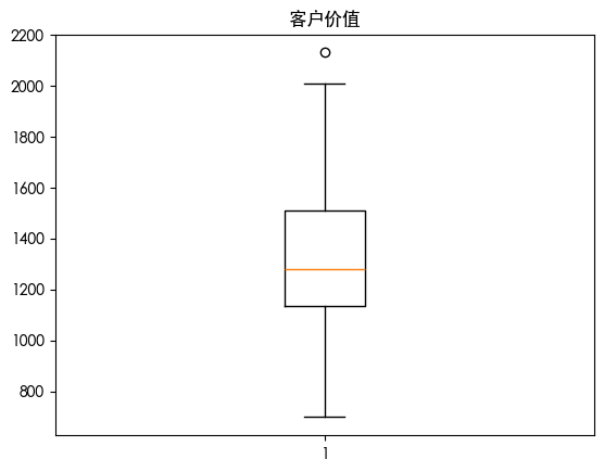
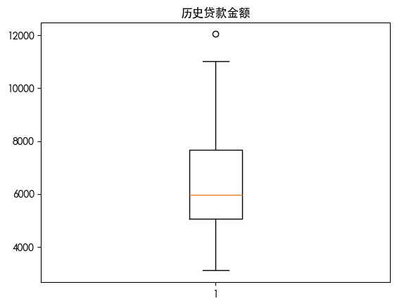
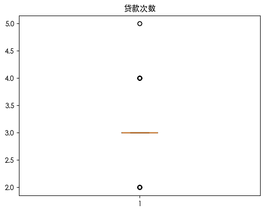
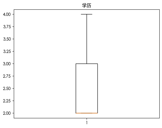
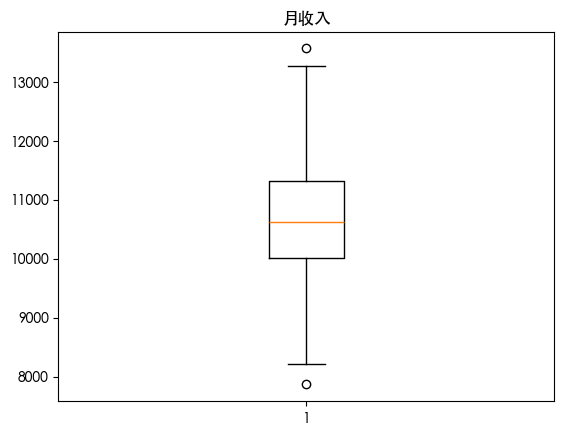
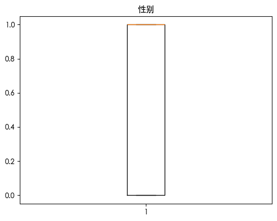
for column in df.columns:
    plt.boxplot(df[column])
    plt.title(column)
    plt.show()

数据划分

from sklearn.model_selection import train_test_split
from sklearn.metrics import mean_squared_error, r2_score

X = df.drop(columns=['客户价值'])
Y = df['客户价值']

x_train, x_test, y_train, y_test = train_test_split(X, Y, test_size=0.2, random_state=42)

多元线性回归

from sklearn.linear_model import LinearRegression

lr = LinearRegression()
lr.fit(x_train, y_train)
y_pred = lr.predict(x_test)

print('mse:', mean_squared_error(y_test, y_pred))
print('r2:', r2_score(y_test, y_pred))

mse: 24535.02941821733
r2: 0.5802551330031818

lr.coef_

array([5.99175873e-02, 1.01030266e+02, 1.19661451e+02, 5.92067892e-02,1.41533251e+01])

import statsmodels.api as sm

X2 = sm.add_constant(X)
est = sm.OLS(Y, X2).fit()
est.summary()

OLS Regression Results

指标	值
Dep. Variable	客户价值
R-squared	0.571
Adj. R-squared	0.553
Model	OLS
Method	Least Squares
F-statistic	32.44
Prob (F-statistic)	6.41e-21
Log-Likelihood	-843.50
No. Observations	128
Df Residuals	122
Df Model	5
Covariance Type	nonrobust
AIC	1699
BIC	1716
Date	Fri, 19 Sep 2025
Time	09:57:49

---

回归系数

| 变量 | coef | std err | t | P>|t| | [0.025 | 0.975] |
|——|——-|———|——|——|——–|——–|
| const | -208.4200 | 163.810 | -1.272 | 0.206 | -532.699 | 115.859 |
| 历史贷款金额 | 0.0571 | 0.010 | 5.945 | 0.000 | 0.038 | 0.076 |
| 贷款次数 | 96.1723 | 25.962 | 3.704 | 0.000 | 44.778 | 147.567 |
| 学历 | 113.4520 | 37.909 | 2.993 | 0.003 | 38.406 | 188.498 |
| 月收入 | 0.0561 | 0.019 | 2.941 | 0.004 | 0.018 | 0.094 |
| 性别 | 1.9787 | 32.286 | 0.061 | 0.951 | -61.934 | 65.891 |

---

诊断统计量

指标	值
Omnibus	1.597
Prob(Omnibus)	0.450
Jarque-Bera (JB)	1.538
Prob(JB)	0.464
Skew	0.264
Kurtosis	2.900
Durbin-Watson	2.155
Cond. No.	1.28e+05

随机森林

from sklearn.ensemble import RandomForestRegressor

rm = RandomForestRegressor()
rm.fit(x_train, y_train)
y_pred = rm.predict(x_test)

print('mse:', mean_squared_error(y_test, y_pred))
print('r2:', r2_score(y_test, y_pred))

mse: 18652.006080769228
r2: 0.6809017964419799

feature_importance = pd.DataFrame({
    "feature": x_train.columns,
    "importance": rm.feature_importances_
}).sort_values(by="importance", ascending=False)
print(feature_importance)

feature	importance
历史贷款金额	0.404590
月收入	0.362695
贷款次数	0.130046
学历	0.073263
性别	0.029405

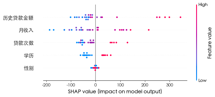
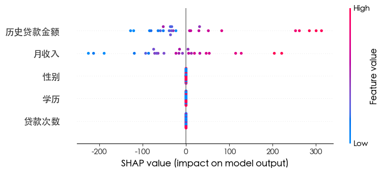
import shap

explainer = shap.TreeExplainer(rm)
shap_values = explainer.shap_values(x_test)

shap.summary_plot(shap_values, x_test)

XGBoost

from xgboost import XGBRegressor

xgb = XGBRegressor(random_state=42)
xgb.fit(x_train, y_train)
y_pred = xgb.predict(x_test)

print("MSE:", mean_squared_error(y_test, y_pred))
print("r2:", r2_score(y_test, y_pred))

MSE: 32402.514511845002
r2: 0.4456583315103658

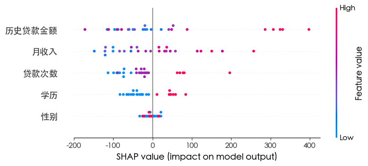
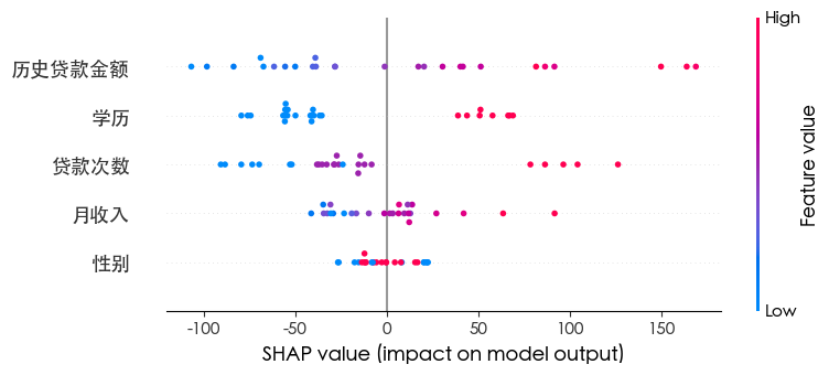
import shap

explainer = shap.TreeExplainer(xgb)
shap_values = explainer.shap_values(x_test)

shap.summary_plot(shap_values, x_test)

KNN

from sklearn.neighbors import KNeighborsRegressor

knn = KNeighborsRegressor(n_neighbors=8)
knn.fit(x_train, y_train)
y_pred = knn.predict(x_test)

print("MSE:", mean_squared_error(y_test, y_pred))
print("r2:", r2_score(y_test, y_pred))

MSE: 20527.141826923078
r2: 0.6488220059125291

import shap
import numpy as np

# 预测函数
f = lambda X: knn.predict(X)

# 选取一部分训练数据作为背景数据
background = x_train.sample(50, random_state=42)

explainer = shap.KernelExplainer(f, background)

shap_values = explainer.shap_values(x_test[:50])  

shap.summary_plot(shap_values, x_test[:50])

SVM

from sklearn.preprocessing import StandardScaler
from sklearn.svm import SVR
from sklearn.pipeline import Pipeline

svr_pipeline = Pipeline([
    ('scaler', StandardScaler()),
    ('svr', SVR(kernel='rbf', C=100, gamma='scale'))
])

svr_pipeline.fit(x_train, y_train)
y_pred = svr_pipeline.predict(x_test)

print("MSE:", mean_squared_error(y_test, y_pred))
print("r2:", r2_score(y_test, y_pred))

MSE: 26681.700620075168
r2: 0.5435299185047356

import shap
import numpy as np

# 预测函数
f = lambda X: svr_pipeline.predict(X)

# 选取一部分训练数据作为背景数据
background = x_train.sample(50, random_state=42)

explainer = shap.KernelExplainer(f, background)

shap_values = explainer.shap_values(x_test[:50])  

shap.summary_plot(shap_values, x_test[:50])