数据来源 https://www.kaggle.com/datasets/mirichoi0218/insurance/data
数据描述 About Dataset
Content
age: age of primary beneficiary
sex: insurance contractor gender, female, male
bmi: Body mass index, providing an understanding of body, weights that are relatively high or low relative to height,
children: Number of children covered by health insurance / Number of dependents
smoker: Smoking
region: the beneficiary’s residential area in the US, northeast, southeast, southwest, northwest.
charges: Individual medical costs billed by health insurance
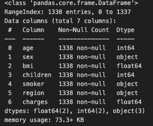
过程 导入库 1 2 3 4 5 6 7 8 9 10 11 12 import pandas as pd import pandas as pd import numpy as np import seaborn as sns import matplotlib.pyplot as plt %matplotlib inline from sklearn.model_selection import train_test_split from sklearn.preprocessing import StandardScaler, OneHotEncoder from sklearn.compose import ColumnTransformer from sklearn.pipeline import Pipeline from sklearn.linear_model import LinearRegression from sklearn.metrics import mean_squared_error, r2_score
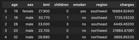
数据查看 1 2 df = pd.read_csv('insurance.csv' )df.head()
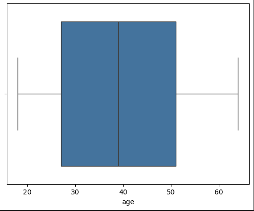
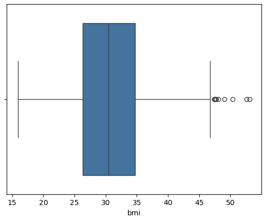
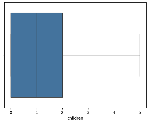
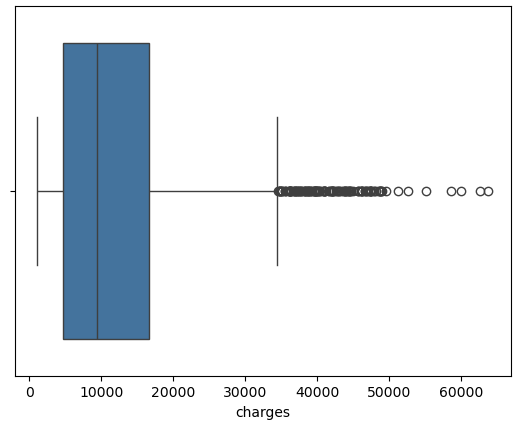
EDA 1 2 3 4 5 num_cols = df.select_dtypes(include=[np.number]).columns.tolist() for col in num_cols: sns.boxplot(x=col, data=df ) plt.show()
可以看到 bmi有异常值
1 2 3 4 from scipy.stats import mstats df ['bmi' ] = mstats.winsorize(df ['bmi' ], limits=[0.05, 0.05])
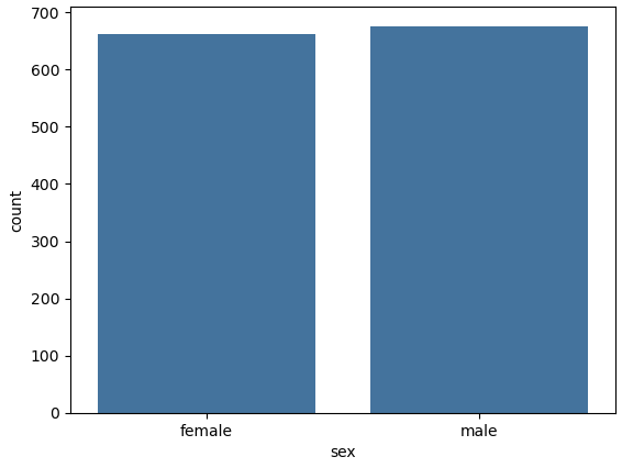
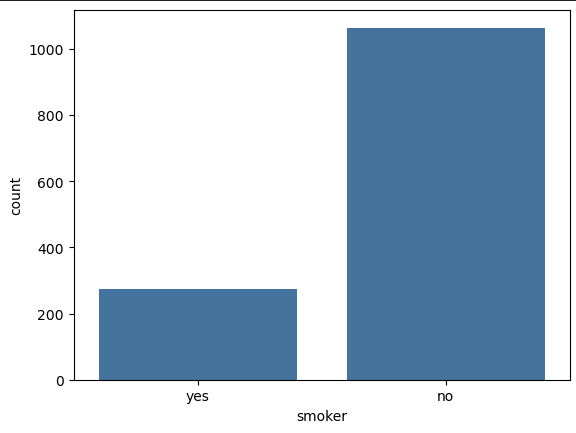
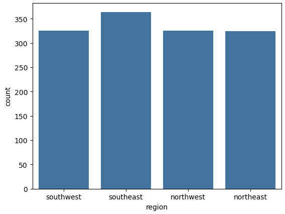
1 2 3 4 5 object_cols = df.select_dtypes(include=['object' ]).columns.tolist() for col in object_cols: sns.countplot(x=col, data=df ) plt.show()
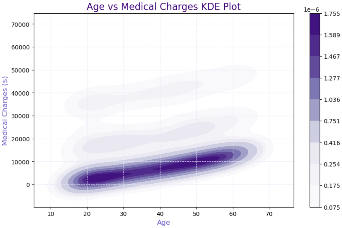
1 2 3 4 5 6 7 8 9 10 11 12 13 14 15 16 17 plt.figure(figsize=(10, 6)) sns.kdeplot( data=df , x="age" , y="charges" , cmap="Purples" , shade=True, cbar=True ) plt.title("Age vs Medical Charges KDE Plot" , fontsize=16, color='indigo' ) plt.xlabel("Age" , fontsize=12, color='slateblue' ) plt.ylabel("Medical Charges ($)" , fontsize=12, color='slateblue' ) plt.grid(True, color='lavender' , linestyle='--' ) plt.show()
可以看到 费用与年龄的关系不大
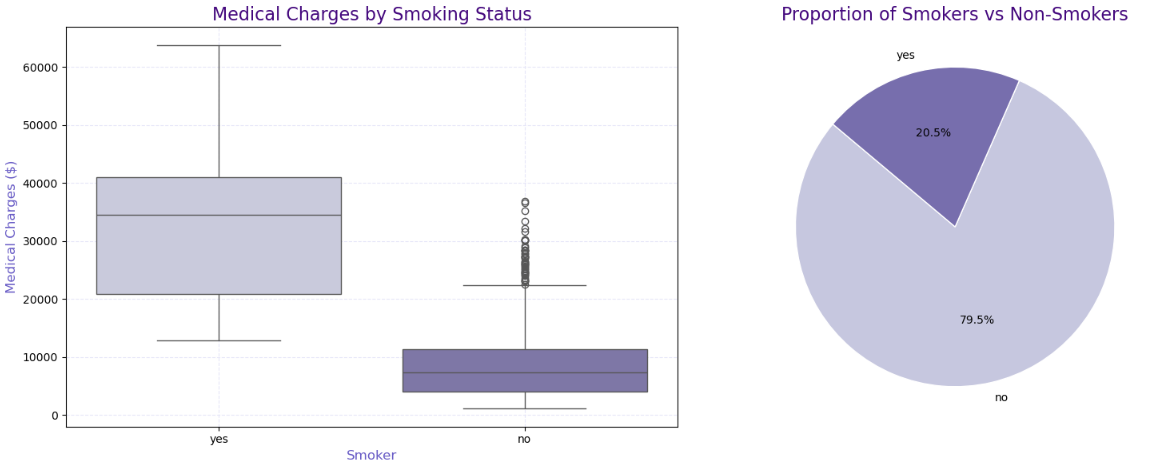
1 2 3 4 5 6 7 8 9 10 11 12 13 14 15 16 17 18 19 20 21 22 23 24 25 26 27 28 29 30 fig, axes = plt.subplots(1, 2, figsize=(16, 6)) colors = sns.color_palette("Purples" , 2) sns.boxplot( ax=axes[0], data=df , x="smoker" , y="charges" , palette="Purples" ) axes[0].set_title("Medical Charges by Smoking Status" , fontsize=16, color='indigo' ) axes[0].set_xlabel("Smoker" , fontsize=12, color='slateblue' ) axes[0].set_ylabel("Medical Charges ($)" , fontsize=12, color='slateblue' ) axes[0].grid(True, linestyle='--' , color='lavender' ) smoker_counts = df ['smoker' ].value_counts() axes[1].pie( smoker_counts, labels=smoker_counts.index, autopct='%1.1f%%' , colors=colors, startangle=140, wedgeprops={'edgecolor' : 'white' } ) axes[1].set_title("Proportion of Smokers vs Non-Smokers" , fontsize=16, color='indigo' ) plt.tight_layout() plt.show()
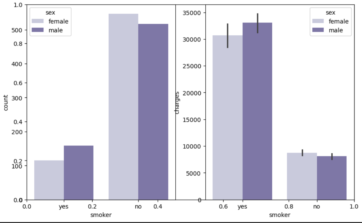
1 2 3 4 5 6 plt.subplots(figsize=(10, 6)) plt.subplot(1, 2, 1) sns.countplot(x='smoker' , data=df ,hue='sex' , palette='Purples' ) plt.subplot(1, 2, 2) sns.barplot(x='smoker' ,y = 'charges' , data=df ,hue='sex' , palette='Purples' ) plt.show()
可以看到 调查者中不吸烟的占大多数 吸烟者中 男性较多 并且 不吸烟的人医疗费用远小于吸烟者
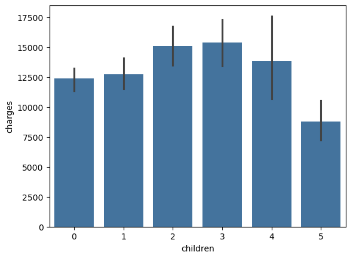
1 2 sns.barplot(x='children' ,y = 'charges' , data=df ) plt.show()
可以看到 有3个孩子的人医疗费用最高 不过我认为 孩子越多费用越高 不过那4和5比3要低 可能因为幸存者偏差:负担的费用过高而破产、自杀、没被记录所导致的
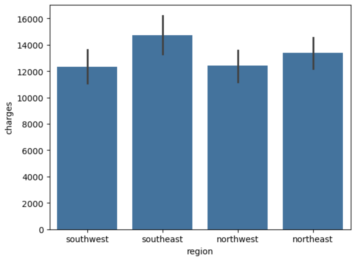
1 2 sns.barplot(x='region' , y='charges' ,data=df ) plt.show()
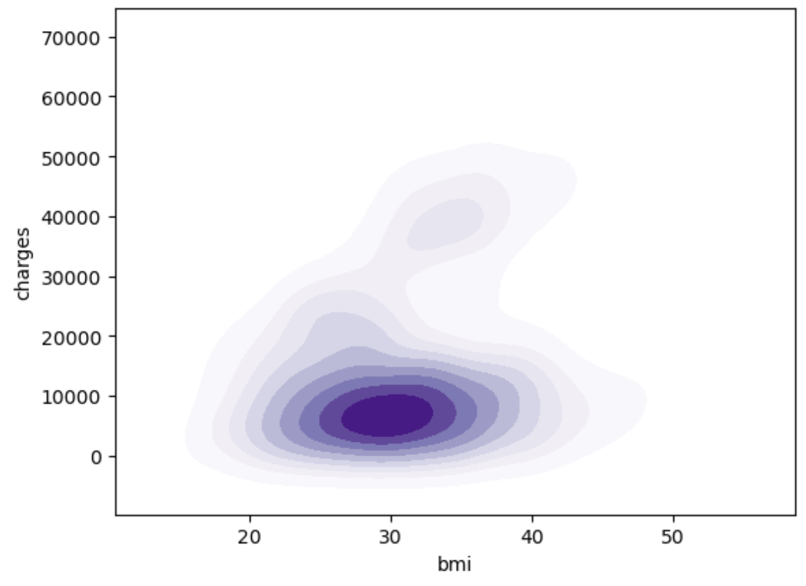
1 2 3 4 5 6 7 8 sns.kdeplot( x='bmi' , y='charges' , shade=True, cmap='Purples' , data=df ) plt.show()
可以看到 大部份人的bmi指数在20~40之间 且费用都在10000左右 通过查询得知 bmi指数在18.5~24.9之间为正常范围 由此得知 现在人们的bmi指数普遍偏高
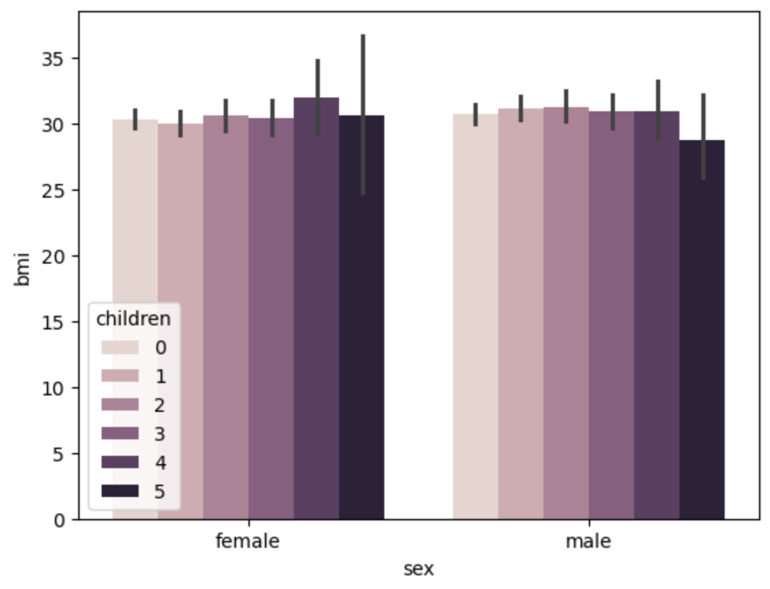
1 2 sns.barplot(x='sex' ,y = 'bmi' ,hue='children' ,data=df ) plt.show()
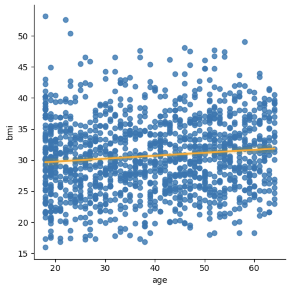
1 2 sns.lmplot(x='age' ,y = 'bmi' ,data=df , line_kws={'color' :'orange' }) plt.show()
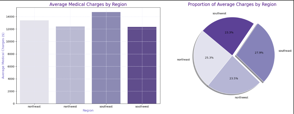
1 2 3 4 5 6 7 8 9 10 11 12 13 14 15 16 17 18 19 20 21 22 23 24 25 26 27 28 29 30 31 32 33 34 35 36 37 average_charges_by_region = df.groupby('region' )['charges' ].mean().reset_index() fig, axes = plt.subplots(1, 2, figsize=(16, 6)) colors = sns.color_palette("Purples" , len(average_charges_by_region)) sns.barplot( ax=axes[0], data=average_charges_by_region, x="region" , y="charges" , palette="Purples" ) axes[0].set_title("Average Medical Charges by Region" , fontsize=16, color='indigo' ) axes[0].set_xlabel("Region" , fontsize=12, color='slateblue' ) axes[0].set_ylabel("Average Medical Charges ($)" , fontsize=12, color='slateblue' ) axes[0].grid(True, linestyle='--' , color='lavender' ) charges = average_charges_by_region['charges' ] regions = average_charges_by_region['region' ] explode = [0.1 if i == charges.idxmax() else 0 for i in range(len(charges))] axes[1].pie( charges, labels=regions, autopct='%1.1f%%' , colors=colors, explode=explode, shadow=True, startangle=140, wedgeprops={'edgecolor' : 'white' } ) axes[1].set_title("Proportion of Average Charges by Region" , fontsize=16, color='indigo' ) plt.tight_layout() plt.show()
数据划分 1 2 3 4 X = df.drop(columns=['charges' ]) y = df ['charges' ] X_train, X_test, y_train, y_test = train_test_split(X, y, test_size=0.2, random_state=42)
特征工程 数值型 归一化
1 2 3 4 5 6 7 num_cols = ['age' , 'bmi' , 'children' ] obj_cols = ['sex' , 'smoker' , 'region' ] preprocessor = ColumnTransformer([ ('scale_num' , StandardScaler(), num_cols), ('encode_obj' , OneHotEncoder(), obj_cols) ])
模型建立(线性回归) 1 2 3 4 5 6 7 preprocessor.fit(X_train) X_train_processed = preprocessor.transform(X_train) X_test_processed = preprocessor.transform(X_test) model = LinearRegression() model.fit(X_train_processed, y_train)
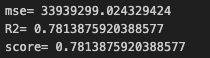
1 2 3 4 5 6 7 8 9 y_pred = model.predict(X_test_processed) mse = mean_squared_error(y_test, y_pred) r2 = r2_score(y_test, y_pred) score = model.score(X_test_processed, y_test) print ("mse =" , mse)print ("R2 =" , r2)print ("score =" , score)
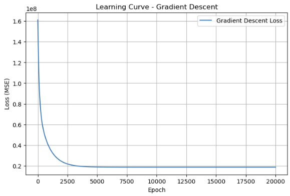
使用不同的优化算法进行优化 梯度下降 1 2 3 4 5 6 7 8 9 10 11 12 13 14 15 16 17 18 19 20 21 22 23 24 25 26 27 28 29 30 31 32 33 34 35 36 37 38 39 40 41 42 43 44 X_train_array = X_train_processed X_test_array = X_test_processed results = {} def gradient_descent(X, y, lr=0.01, n_epochs=1000): m, n = X.shape w = np.random.randn(n) b = 0 losses = [] for epoch in range(n_epochs): y_pred = X @ w + b error = y_pred - y grad_w = (1/m) * X.T @ error grad_b = (1/m) * np.sum(error) w -= lr * grad_w b -= lr * grad_b loss = (1/(2*m)) * np.sum(error**2) losses.append(loss) return w, b, losses w_gd, b_gd, losses_gd = gradient_descent(X_train_array, y_train.values, lr=0.002, n_epochs=20000) y_pred_gd = X_test_array @ w_gd + b_gd results['Gradient Descent' ] = { 'MSE' : mean_squared_error(y_test, y_pred_gd), 'R2' : r2_score(y_test, y_pred_gd) } results_df = pd.DataFrame(results).T print (results_df)plt.figure(figsize=(8, 5)) plt.plot(range(1, len(losses_gd)+1), losses_gd, label='Gradient Descent Loss' ) plt.xlabel('Epoch' ) plt.ylabel('Loss (MSE)' ) plt.title('Learning Curve - Gradient Descent' ) plt.legend() plt.grid(True) plt.show()
牛顿法 1 2 3 4 5 6 7 8 9 10 11 12 13 14 15 16 X_train_bias = np.hstack([X_train_array, np.ones((X_train_array.shape[0 ], 1 ))]) X_test_bias = np.hstack([X_test_array, np.ones((X_test_array.shape[0 ], 1 ))]) XTX = X_train_bias.T @ X_train_bias XTy = X_train_bias.T @ y_train.values w_newton = np.linalg.pinv(XTX) @ XTy y_pred_newton = X_test_bias @ w_newton results["Newton's Method" ] = { 'MSE' : mean_squared_error(y_test, y_pred_newton), 'R2' : r2_score(y_test, y_pred_newton) } results_df = pd.DataFrame(results).T print (results_df)
SGDRegressor 1 2 3 4 5 6 7 8 9 10 from sklearn.linear_model import SGDRegressor sgd_model = SGDRegressor(penalty=None,max_iter=10000, learning_rate='adaptive' , eta0=0.001, random_state=42) sgd_model.fit(X_train_array, y_train) y_pred_sgd = sgd_model.predict(X_test_array) results['SGDRegressor (sklearn)' ] = { 'MSE' : mean_squared_error(y_test, y_pred_sgd), 'R2' : r2_score(y_test, y_pred_sgd) }
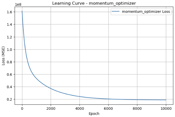
动量法 1 2 3 4 5 6 7 8 9 10 11 12 13 14 15 16 17 18 19 20 21 22 23 24 25 26 27 28 29 30 31 32 33 34 35 36 37 38 39 40 41 42 43 44 45 46 47 48 49 def momentum_optimizer(X, y, lr=0.01, n_epochs=1000, beta=0.9): m, n = X.shape w = np.random.randn(n) b = 0 v_w = np.zeros(n) v_b = 0 losses = [] for epoch in range(n_epochs): y_pred = X @ w + b error = y_pred - y grad_w = (1/m) * (X.T @ error) grad_b = (1/m) * np.sum(error) v_w = beta * v_w + (1 - beta) * grad_w v_b = beta * v_b + (1 - beta) * grad_b w -= lr * v_w b -= lr * v_b loss = (1/(2*m)) * np.sum(error**2) losses.append(loss) return w, b, losses w_momentum, b_momentum, losses_momentum = momentum_optimizer(X_train_array, y_train.values, lr=0.001, n_epochs=10000, beta=0.9) y_pred_momentum = X_test_array @ w_momentum + b_momentum results['momentum_optimizer' ] = { 'MSE' : mean_squared_error(y_test, y_pred_momentum), 'R2' : r2_score(y_test, y_pred_momentum) } plt.figure(figsize=(8, 5)) plt.plot(range(1, len(losses_momentum)+1), losses_momentum, label='momentum_optimizer Loss' ) plt.xlabel('Epoch' ) plt.ylabel('Loss (MSE)' ) plt.title('Learning Curve - momentum_optimizer' ) plt.legend() plt.grid(True) plt.show()
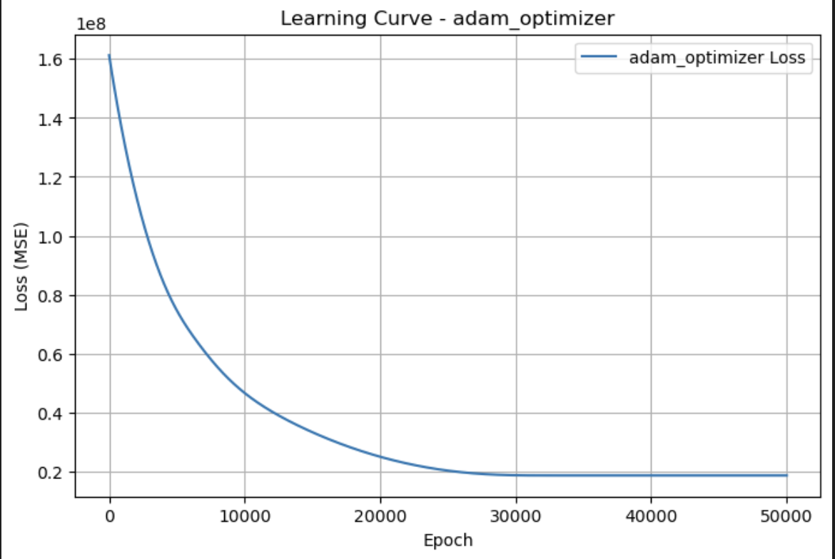
Adam优化器 1 2 3 4 5 6 7 8 9 10 11 12 13 14 15 16 17 18 19 20 21 22 23 24 25 26 27 28 29 30 31 32 33 34 35 36 37 38 39 40 41 42 43 44 45 46 47 48 49 50 51 52 53 54 55 56 57 58 59 def adam_optimizer(X, y, lr=0.001, n_epochs=1000, beta1=0.9, beta2=0.999, epsilon=1e-8): m, n = X.shape w = np.random.randn(n) b = 0 m_w = np.zeros(n) v_w = np.zeros(n) m_b = 0 v_b = 0 losses = [] for epoch in range(n_epochs): y_pred = X @ w + b error = y_pred - y grad_w = (1/m) * (X.T @ error) grad_b = (1/m) * np.sum(error) m_w = beta1 * m_w + (1 - beta1) * grad_w v_w = beta2 * v_w + (1 - beta2) * (grad_w ** 2) m_b = beta1 * m_b + (1 - beta1) * grad_b v_b = beta2 * v_b + (1 - beta2) * (grad_b ** 2) m_w_hat = m_w / (1 - beta1 ** (epoch + 1)) v_w_hat = v_w / (1 - beta2 ** (epoch + 1)) m_b_hat = m_b / (1 - beta1 ** (epoch + 1)) v_b_hat = v_b / (1 - beta2 ** (epoch + 1)) w -= lr * m_w_hat / (np.sqrt(v_w_hat) + epsilon) b -= lr * m_b_hat / (np.sqrt(v_b_hat) + epsilon) loss = (1/(2*m)) * np.sum(error**2) losses.append(loss) return w, b, losses w_adam, b_adam, losses_adam = adam_optimizer(X_train_array, y_train.values, lr=0.0001, n_epochs=50000,beta1=0.85) y_pred_adam = X_test_array @ w_adam + b_adam results['adam_optimizer' ] = { 'MSE' : mean_squared_error(y_test, y_pred_adam), 'R2' : r2_score(y_test, y_pred_adam) } plt.figure(figsize=(8, 5)) plt.plot(range(1, len(losses_adam)+1), losses_adam, label='adam_optimizer Loss' ) plt.xlabel('Epoch' ) plt.ylabel('Loss (MSE)' ) plt.title('Learning Curve - adam_optimizer' ) plt.legend() plt.grid(True) plt.show()
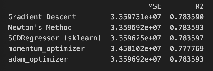
1 2 results_df = pd.DataFrame(results).T print (results_df)
使用随机森林预测 1 2 3 4 5 6 7 8 9 10 11 12 from sklearn.ensemble import RandomForestRegressor rf_model = RandomForestRegressor(n_estimators=100, random_state=42) rf_model.fit(X_train_processed, y_train) y_pred_rf = rf_model.predict(X_test_array) mse_rf = mean_squared_error(y_test, y_pred_rf) r2_rf = r2_score(y_test, y_pred_rf) print (f"Random Forest MSE: {mse_rf:.4f}" )print (f"Random Forest R2: {r2_rf:.4f}" )
Random Forest MSE: 21083936.2878
贝叶斯优化 1 2 3 4 5 6 7 8 9 10 11 12 13 14 15 16 17 18 19 20 21 22 23 24 25 26 27 28 29 30 31 32 33 34 from hyperopt import fmin, tpe, hp, STATUS_OK, Trials def objective(params): model = RandomForestRegressor( n_estimators=int(params['n_estimators' ]), max_depth=int(params['max_depth' ]), min_samples_split=int(params['min_samples_split' ]), min_samples_leaf=int(params['min_samples_leaf' ]), random_state=42 ) model.fit(X_train_processed, y_train) y_pred = model.predict(X_test_processed) mse = mean_squared_error(y_test, y_pred) rmse = np.sqrt(mse) return {'loss' : rmse,'status' : STATUS_OK} space = { 'n_estimators' : hp.quniform('n_estimators' , 50, 200, 1), 'max_depth' : hp.quniform('max_depth' , 5, 20, 1), 'min_samples_split' : hp.quniform('min_samples_split' , 2, 10, 1), 'min_samples_leaf' : hp.quniform('min_samples_leaf' , 1, 4, 1) } tpe_algorithm = tpe.suggest trials = Trials() best = fmin(fn=objective, space=space, algo=tpe_algorithm, max_evals=20, trials=trials) print ("Best parameters found: " , best)
100%|██████████| 20/20 [00:02<00:00, 6.72trial/s, best loss: 4357.951533549515]
1 2 3 4 5 6 7 8 9 10 11 12 13 14 15 best_model = RandomForestRegressor( n_estimators=int(best['n_estimators' ]), max_depth=int(best['max_depth' ]), min_samples_split=int(best['min_samples_split' ]), min_samples_leaf=int(best['min_samples_leaf' ]), random_state=42 ) best_model.fit(X_train_processed, y_train) y_pred = best_model.predict(X_test_processed) mse = mean_squared_error(y_test, y_pred) rmse = np.sqrt(mse) R2 = r2_score(y_test, y_pred) print (f"RMSE: {rmse}" )print (f"R2: {R2}" )
RMSE: 4357.951533549515
网格优化 1 2 3 4 5 6 7 8 9 10 11 12 13 14 15 16 17 18 19 20 21 22 23 24 from sklearn.model_selection import GridSearchCV param_grid = { 'n_estimators' : [100, 200, 300], 'max_depth' : [10, 20, None], 'min_samples_split' : [2, 5, 10], 'min_samples_leaf' : [1, 2, 4], 'max_features' : ['sqrt' , 'log2' ] } grid_search = GridSearchCV( estimator=rf_model, param_grid=param_grid, cv=5, n_jobs=-1, verbose=2 ) grid_search.fit(X_train_processed, y_train) print ("最优参数:" , grid_search.best_params_)print ("最优得分:" , grid_search.best_score_)
最优参数: {‘max_depth’: 10, ‘max_features’: ‘sqrt’, ‘min_samples_leaf’: 2, ‘min_samples_split’: 2, ‘n_estimators’: 300}
综上 无论是线性回归还是随机森林 在进行优化后 他们的分数都至少上升了1% 说明使用优化器进行优化是有效果的