商业数据分析--信用评分卡模型

声明

本文代码均保存在
https://github.com/super-213/business_data_analysis
有需要的可以自行下载

查看数据

df = pd.read_excel('信用评分卡模型.xlsx')
df.head()

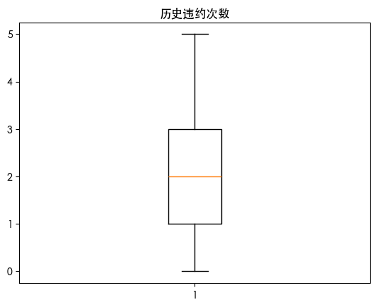
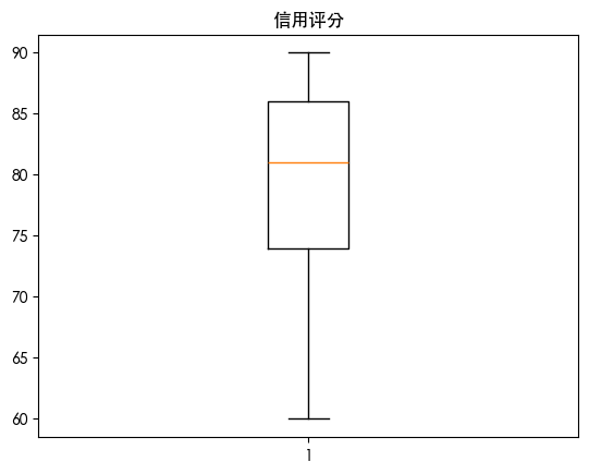
月收入	年龄	性别	历史授信额度	历史违约次数	信用评分
7783	29	0	32274	3	73
7836	40	1	6681	4	72
6398	25	0	26038	2	74
6483	23	1	24584	4	65
5167	23	1	6710	3	73

缺失值处理

df.isnull().sum()

字段	缺失值数量
月收入	0
年龄	0
性别	0
历史授信额度	0
历史违约次数	0
信用评分	0

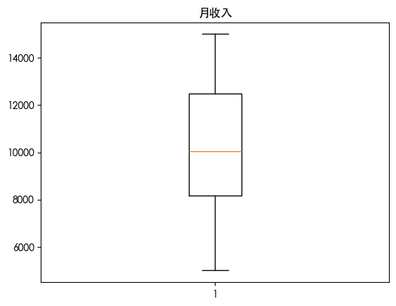
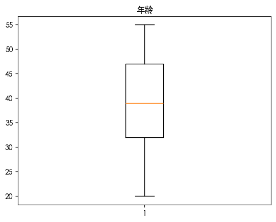
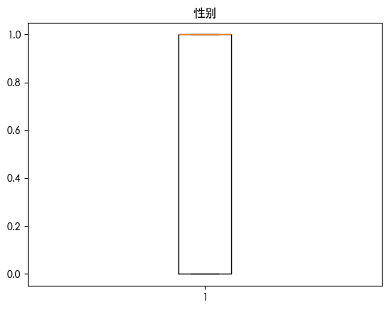
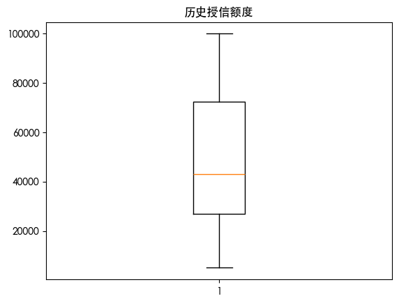
异常值处理

for col in df.columns:
    plt.boxplot(df[col])
    plt.title(col)
    plt.show()

数据划分

from sklearn.model_selection import train_test_split
X = df.drop(columns=['信用评分'])
y = df['信用评分']
X_train, X_test, y_train, y_test = train_test_split(X, y, test_size=0.2, random_state=42)

XGBoost

from xgboost import XGBRegressor

xgb = XGBRegressor(objective='reg:squarederror', random_state=42)
xgb.fit(X_train, y_train)
y_pred = xgb.predict(X_test)

from sklearn.metrics import mean_squared_error, r2_score
mse = mean_squared_error(y_test, y_pred)
r2 = r2_score(y_test, y_pred)
print(f'Mean Squared Error: {mse}')
print(f'R^2 Score: {r2}')

Mean Squared Error: 30.737820683092288
R^2 Score: 0.5528881678156692

网格优化

from sklearn.model_selection import GridSearchCV  
parameters = {'max_depth': [1, 3, 5], 'n_estimators': [50, 100, 150], 'learning_rate': [0.01, 0.05, 0.1, 0.2]}  # 指定模型中参数的范围
xgb_best = XGBRegressor()
grid_search = GridSearchCV(xgb_best, parameters, cv=5, scoring='neg_mean_squared_error')  # 5折交叉验证
grid_search.fit(X_train, y_train)
print("Best parameters:", grid_search.best_params_)

best_xgb = grid_search.best_estimator_
y_pred_best = best_xgb.predict(X_test)
mse_best = mean_squared_error(y_test, y_pred_best)
r2_best = r2_score(y_test, y_pred_best)
print(f'Optimized Mean Squared Error: {mse_best}')
print(f'Optimized R^2 Score: {r2_best}')

Best parameters: {‘learning_rate’: 0.05, ‘max_depth’: 3, ‘n_estimators’: 50}

Optimized Mean Squared Error: 22.005304773406532
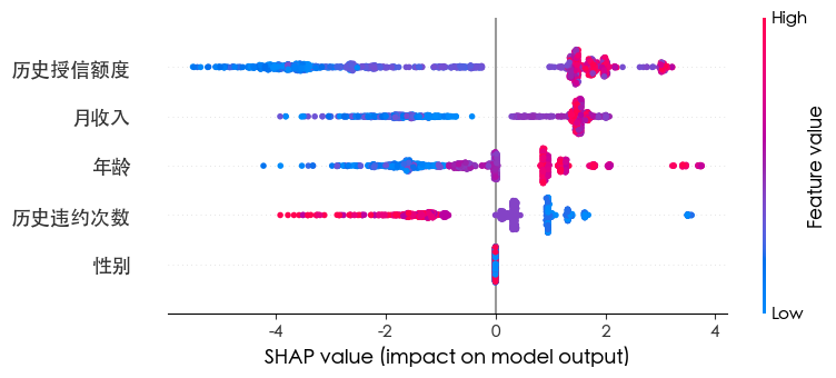
Optimized R^2 Score: 0.6799112000668165

feature_importances = best_xgb.feature_importances_
features = X.columns
importance_df = pd.DataFrame({'Feature': features, 'Importance': feature_importances})
importance_df.sort_values(by='Importance', ascending=False, inplace=True)
importance_df

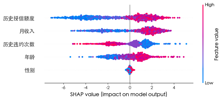
import shap
explainer = shap.Explainer(best_xgb)
shap_values = explainer(X)
shap.summary_plot(shap_values, X)

LGBM

from lightgbm import LGBMRegressor
from sklearn.metrics import mean_squared_error, r2_score

lgbm = LGBMRegressor(random_state=42)
lgbm.fit(X_train, y_train)
y_pred_lgbm = lgbm.predict(X_test)
mse_lgbm = mean_squared_error(y_test, y_pred_lgbm)
r2_lgbm = r2_score(y_test, y_pred_lgbm)
print(f'LightGBM Mean Squared Error: {mse_lgbm}')
print(f'LightGBM R^2 Score: {r2_lgbm}')

feature_importances_lgbm = lgbm.feature_importances_
features = X.columns
importance_df_lgbm = pd.DataFrame({'Feature': features, 'Importance': feature_importances_lgbm})
importance_df_lgbm.sort_values(by='Importance', ascending=False, inplace=True)
importance_df_lgbm

explainer = shap.Explainer(lgbm)
shap_values = explainer(X)
shap.summary_plot(shap_values, X)

LightGBM Mean Squared Error: 25.26260176146583
LightGBM R^2 Score: 0.6325306118554737

随机森林

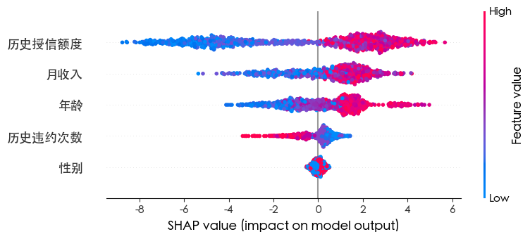
from sklearn.ensemble import RandomForestRegressor

rm = RandomForestRegressor(random_state=42)
rm.fit(X_train, y_train)
y_pred_rm = rm.predict(X_test)
mse_rm = mean_squared_error(y_test, y_pred_rm)
r2_rm = r2_score(y_test, y_pred_rm)
print(f'Random Forest Mean Squared Error: {mse_rm}')
print(f'Random Forest R^2 Score: {r2_rm}')

feature_importances_rm = rm.feature_importances_
features = X.columns
importance_df_rm = pd.DataFrame({'Feature': features, 'Importance': feature_importances_rm})
importance_df_rm.sort_values(by='Importance', ascending=False, inplace=True)
importance_df_rm

explainer = shap.Explainer(rm)
shap_values = explainer(X)
shap.summary_plot(shap_values, X)

Random Forest Mean Squared Error: 22.497981999999997
Random Forest R^2 Score: 0.6727447252627369

LDA

from sklearn.discriminant_analysis import LinearDiscriminantAnalysis

lda = LinearDiscriminantAnalysis()
lda.fit(X_train, y_train)
y_pred_lda = lda.predict(X_test)
mse_lda = mean_squared_error(y_test, y_pred_lda)
r2_lda = r2_score(y_test, y_pred_lda)
print(f'Linear Discriminant Analysis Mean Squared Error: {mse_lda}')
print(f'Linear Discriminant Analysis R^2 Score: {r2_lda}')

feature_importances_lda = lda.coef_[0]
features = X.columns
importance_df_lda = pd.DataFrame({'Feature': features, 'Importance': feature_importances_lda})
importance_df_lda.sort_values(by='Importance', ascending=False, inplace=True)
importance_df_lda

Linear Discriminant Analysis Mean Squared Error: 30.66
Linear Discriminant Analysis R^2 Score: 0.5540201461871341

KNN

from sklearn.neighbors import KNeighborsRegressor

knn = KNeighborsRegressor(n_neighbors=5)
knn.fit(X_train, y_train)
y_pred_knn = knn.predict(X_test)
mse_knn = mean_squared_error(y_test, y_pred_knn)
r2_knn = r2_score(y_test, y_pred_knn)

print(f'KNN Mean Squared Error: {mse_knn}')
print(f'KNN R^2 Score: {r2_knn}')

KNN Mean Squared Error: 25.003800000000002
KNN R^2 Score: 0.6362951380050184

模型横向比较

模型	MSE ↓	R² ↑	特点总结
XGBoost (优化后)	22.01	0.680	树模型，调参后效果最好之一，兼顾偏差与方差，特征重要性可解释性强。
LightGBM	25.26	0.633	与XGBoost类似，但默认参数下稍逊，可能因数据量不大导致优势未显现。
随机森林	22.50	0.673	稳定性高，效果接近XGBoost，调参空间不如Boosting大。
LDA	30.66	0.554	线性判别方法，更适合分类；在回归任务上受限，表现最差。
KNN	25.00	0.636	简单直观，依赖局部邻域；在高维数据中容易过拟合或欠拟合。

差异分析

1. 树模型（XGBoost / LightGBM / 随机森林）表现最佳

   • 它们能捕捉非线性关系，适合处理信用评分这类复杂特征交互的任务。
   • XGBoost 调参后效果最好（R²≈0.68），说明该数据集对树模型的适配性很好。
   • 随机森林 与 XGBoost 表现接近，但略逊，因为 Boosting 更好地优化了偏差。
   • LightGBM 在大数据下优势明显，但在你这种数据量（200左右样本）下未完全发挥。

2. 线性方法（LDA）表现最差

   • 信用评分与特征之间关系并非单纯线性，导致 LDA 只能捕捉有限信息。
   • R²≈0.55，MSE最大，说明解释力有限。

3. KNN 居中但不稳定

   • 表现优于 LDA，但不如树模型。
   • 优点是简单、无需训练；缺点是容易受到特征尺度影响，且在高维空间中“邻近”的意义变弱。

结论

• 最佳模型推荐：XGBoost（调参后）
  兼具预测准确性和可解释性，适合在信用评分建模中作为主力模型。
• 随机森林 可作为备选基准模型，在稳定性上更强，但可解释性略弱。
• LightGBM 如果数据规模增大 可能会超过XGBoost。
• LDA 和 KNN 更适合作为参考或对比，实际预测能力有限。