商业数据分析--员工离职预测模型

声明

本文代码均保存在
https://github.com/super-213/business_data_analysis
有需要的可以自行下载

查看数据

df =pd.read_excel('员工离职预测模型.xlsx')

df.head()

工资	满意度	考核得分	工程数量	月工时	工龄	离职
低	3.8	0.53	2	157	3	1
中	8.0	0.86	5	262	6	1
中	1.1	0.88	7	272	4	1
低	7.2	0.87	5	223	5	1
低	3.7	0.52	2	159	3	1

缺失值处理

df.isnull().sum()

字段	缺失值数量
工资	0
满意度	0
考核得分	0
工程数量	0
月工时	0
工龄	0
离职	0

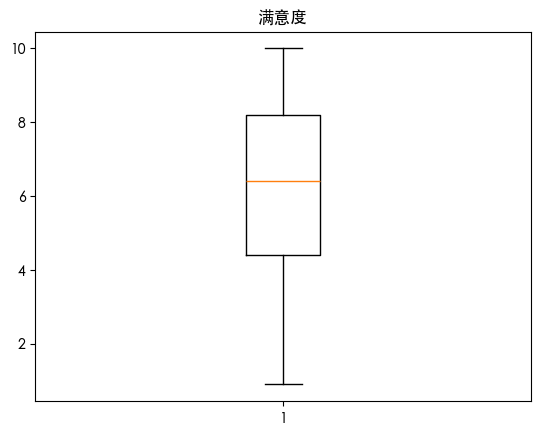
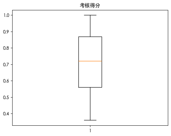
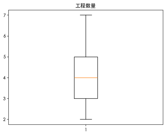
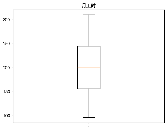
异常值处理

for col in df.select_dtypes(include=['number']).columns:
    plt.boxplot(df[col])
    plt.title(col)
    plt.show()

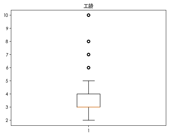
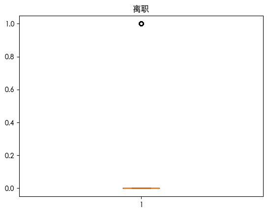
通过上述图表我们发现
离职（目标变量）存在异常值
从上面分析中我们知道离职是0-1变量 这说明离职的样本中 不离职的样本非常多 离职的样本非常少 这导致其把离职的当成了异常值

工龄存在异常值
我们发现大部份人的工龄在2-5年之间 那些被认为是异常值的都是工龄较长的由于我们是要做员工离职预测模型 我认为那些离职的员工有可能是那些工龄年限长的员工 因此我们不能把这个异常值给删除或归一化处理 因此我们将这个异常值给突出保留下来

col = '工龄'

Q1 = df[col].quantile(0.25)
Q3 = df[col].quantile(0.75)
IQR = Q3 - Q1

lower_bound = Q1 - 1.5 * IQR
upper_bound = Q3 + 1.5 * IQR

df[f'{col}_is_outlier'] = ((df[col] < lower_bound) | (df[col] > upper_bound)).astype(int)

特征编码

可以看到 工资特征不是数值型 我们需要对其进行处理

因为初始工资是按照低中高分类的 因此我们直接使用映射将低中高映射为0、1、2 这样还能保留低中高的顺序关系
注意 这里不推荐使用独热编码 因为其会丢失低中高的顺序关系

df['工资'] = df['工资'].map({'低': 0, '中': 1, '高': 2})

数据划分

from sklearn.model_selection import train_test_split

X = df.drop(columns=['离职'])
y = df['离职']

X_train, X_test, y_train, y_test = train_test_split(X, y, test_size=0.2, random_state=42)

决策树

from sklearn.tree import DecisionTreeClassifier
dtc = DecisionTreeClassifier(random_state=42)
dtc.fit(X_train, y_train)
y_pred = dtc.predict(X_test)

from sklearn.metrics import classification_report, confusion_matrix
print(confusion_matrix(y_test, y_pred))
print(classification_report(y_test, y_pred))

实际 \ 预测	0	1
0	900	136
1	150	223

类别	Precision	Recall	F1-Score	Support
0	0.86	0.87	0.86	1036
1	0.62	0.60	0.61	373
accuracy			0.80	1409
macro avg	0.74	0.73	0.74	1409
weighted avg	0.80	0.80	0.80	1409

from sklearn.model_selection import cross_val_score

scores = cross_val_score(dtc, X_train, y_train, cv=5, scoring='accuracy')

print("各折准确率：", scores)
print("平均准确率：%.4f (+/- %.4f)" % (scores.mean(), scores.std() * 2))

各折准确率： [0.97625 0.97833333 0.96958333 0.97541667 0.98 ]
平均准确率：0.9759 (+/- 0.0071)

from sklearn.model_selection import GridSearchCV
from sklearn.tree import DecisionTreeClassifier

param_grid = {
    'max_depth': [3, 5, 7, 10, None],
    'min_samples_split': [2, 5, 10],
    'min_samples_leaf': [1, 2, 4],
    'criterion': ['gini', 'entropy']
}

dtc = DecisionTreeClassifier(random_state=42)

grid_search = GridSearchCV(
    estimator=dtc,
    param_grid=param_grid,
    cv=5,
    scoring='f1',
    n_jobs=-1,           # 使用所有 CPU 核心加速
    verbose=1            # 显示过程
)

grid_search.fit(X_train, y_train)

print("最佳参数：", grid_search.best_params_)
print("最佳交叉验证得分：%.4f" % grid_search.best_score_)

best_dtc = grid_search.best_estimator_
y_pred = best_dtc.predict(X_test)

from sklearn.metrics import classification_report, confusion_matrix
print("\n=== 测试集结果 ===")
print("混淆矩阵：")
print(confusion_matrix(y_test, y_pred))
print("\n分类报告：")
print(classification_report(y_test, y_pred))

最佳参数：
{'criterion': 'entropy', 'max_depth': None, 'min_samples_leaf': 1, 'min_samples_split': 2}

最佳交叉验证得分： 0.9564
混淆矩阵：

实际 \ 预测	0	1
0	2236	38
1	21	705

分类报告：

类别	Precision	Recall	F1-Score	Support
0	0.99	0.98	0.99	2274
1	0.95	0.97	0.96	726
accuracy			0.98	3000
macro avg	0.97	0.98	0.97	3000
weighted avg	0.98	0.98	0.98	3000

随机森林

from sklearn.ensemble import RandomForestClassifier

rm = RandomForestClassifier(random_state=42)
rm.fit(X_train, y_train)
y_pred = rm.predict(X_test)

print(confusion_matrix(y_test, y_pred))
print(classification_report(y_test, y_pred))

实际 \ 预测	0	1
0	2268	6
1	20	706

类别	Precision	Recall	F1-Score	Support
0	0.99	1.00	0.99	2274
1	0.99	0.97	0.98	726
accuracy			0.99	3000
macro avg	0.99	0.98	0.99	3000
weighted avg	0.99	0.99	0.99	3000

scores = cross_val_score(rm, X_train, y_train, cv=5, scoring='accuracy')

print("各折准确率：", scores)
print("平均准确率：%.4f (+/- %.4f)" % (scores.mean(), scores.std() * 2))

各折准确率： [0.99041667 0.99041667 0.98833333 0.99083333 0.99208333]
平均准确率：0.9904 (+/- 0.0024)

GBDT

from sklearn.ensemble import GradientBoostingClassifier

GBDT = GradientBoostingClassifier(random_state=42)
GBDT.fit(X_train, y_train)
y_pred = GBDT.predict(X_test)

print(confusion_matrix(y_test, y_pred))
print(classification_report(y_test, y_pred))

实际 \ 预测	0	1
0	2249	25
1	53	673

类别	Precision	Recall	F1-Score	Support
0	0.98	0.99	0.98	2274
1	0.96	0.93	0.95	726
accuracy			0.97	3000
macro avg	0.97	0.96	0.96	3000
weighted avg	0.97	0.97	0.97	3000

各折准确率： [0.97333333 0.97625 0.97708333 0.97708333 0.97458333]
平均准确率：0.9757 (+/- 0.0030)

朴素贝叶斯

from sklearn.naive_bayes import GaussianNB

nb = GaussianNB()
nb.fit(X_train, y_train)

y_pred_nb = nb.predict(X_test)
y_pred_proba = nb.predict_proba(X_test)[:, 1]  # 离职概率（正类概率）

print("混淆矩阵：")
print(confusion_matrix(y_test, y_pred_nb))
print("\n分类报告：")
print(classification_report(y_test, y_pred_nb))

print("\n前5个样本的离职概率：", y_pred_proba[:5])

实际 \ 预测	0	1
0	2071	203
1	293	433

类别	Precision	Recall	F1-Score	Support
0	0.88	0.91	0.89	2274
1	0.68	0.60	0.64	726
accuracy			0.83	3000
macro avg	0.78	0.75	0.76	3000
weighted avg	0.83	0.83	0.83	3000

前5个样本的离职概率：
[0.0299, 0.0785, 0.0041, 0.6395, 0.1225]

LDA

from sklearn.discriminant_analysis import LinearDiscriminantAnalysis

LDA = LinearDiscriminantAnalysis()
LDA.fit(X_train, y_train)
y_pred_lda = LDA.predict(X_test)
y_pred_proba_lda = LDA.predict_proba(X_test)[:, 1]

print("混淆矩阵：")
print(confusion_matrix(y_test, y_pred_lda))
print("\n分类报告：")
print(classification_report(y_test, y_pred_lda))

实际 \ 预测	0	1
0	2096	178
1	523	203

类别	Precision	Recall	F1-Score	Support
0	0.80	0.92	0.86	2274
1	0.53	0.28	0.37	726
accuracy			0.77	3000
macro avg	0.67	0.60	0.61	3000
weighted avg	0.74	0.77	0.74	3000

XGBoost

from xgboost import XGBClassifier

xgb = XGBClassifier()
xgb.fit(X_train, y_train)
y_pred_xgb = xgb.predict(X_test)
y_pred_proba_xgb = xgb.predict_proba(X_test)[:, 1]

print("混淆矩阵：")
print(confusion_matrix(y_test, y_pred_xgb))
print("\n分类报告：")
print(classification_report(y_test, y_pred_xgb))

实际 \ 预测	0	1
0	2260	14
1	29	697

类别	Precision	Recall	F1-Score	Support
0	0.99	0.99	0.99	2274
1	0.98	0.96	0.97	726
accuracy			0.99	3000
macro avg	0.98	0.98	0.98	3000
weighted avg	0.99	0.99	0.99	3000