商业数据分析--肿瘤数据

声明
本文代码均保存在
https://github.com/super-213/business_data_analysis
有需要的可以自行下载
查看数据
1 | df = pd.read_excel('肿瘤数据.xlsx') |
| 最大周长 | 最大凹陷度 | 平均凹陷度 | 最大面积 | 最大半径 | 平均灰度值 | 肿瘤性质 |
|---|---|---|---|---|---|---|
| 184.60 | 0.2654 | 0.14710 | 2019.0 | 25.38 | 17.33 | 0 |
| 158.80 | 0.1860 | 0.07017 | 1956.0 | 24.99 | 23.41 | 0 |
| 152.50 | 0.2430 | 0.12790 | 1709.0 | 23.57 | 25.53 | 1 |
| 98.87 | 0.2575 | 0.10520 | 567.7 | 14.91 | 26.50 | 0 |
| 152.20 | 0.1625 | 0.10430 | 1575.0 | 22.54 | 16.67 | 0 |
缺失值处理
1 | df.isnull().sum() |
| 字段 | 缺失值数量 |
|---|---|
| 最大周长 | 0 |
| 最大凹陷度 | 0 |
| 平均凹陷度 | 0 |
| 最大面积 | 0 |
| 最大半径 | 0 |
| 平均灰度值 | 0 |
| 肿瘤性质 | 0 |
异常值处理
1 | for col in df.columns: |
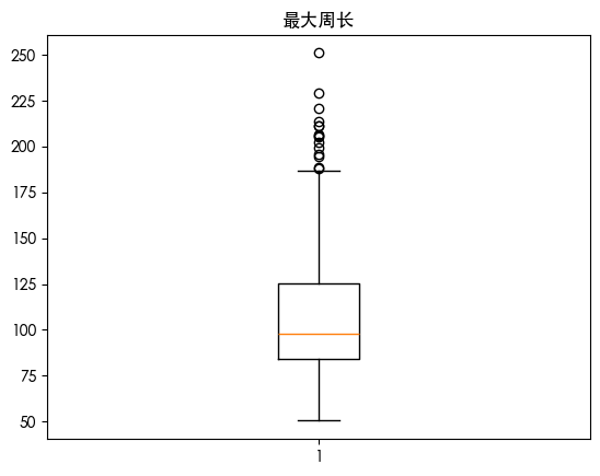
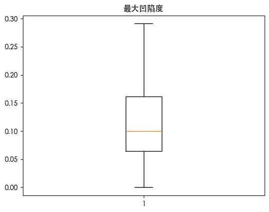
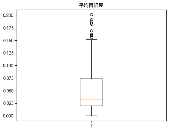
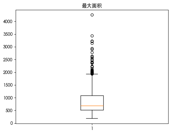
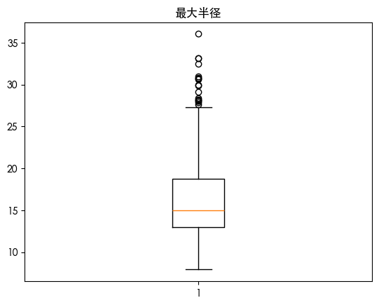
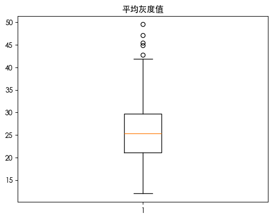
发现用四分位数发现存在一些异常值 朴素贝叶斯是对异常值敏感的 我们可视化数据的分布情况
1 | import seaborn as sns |
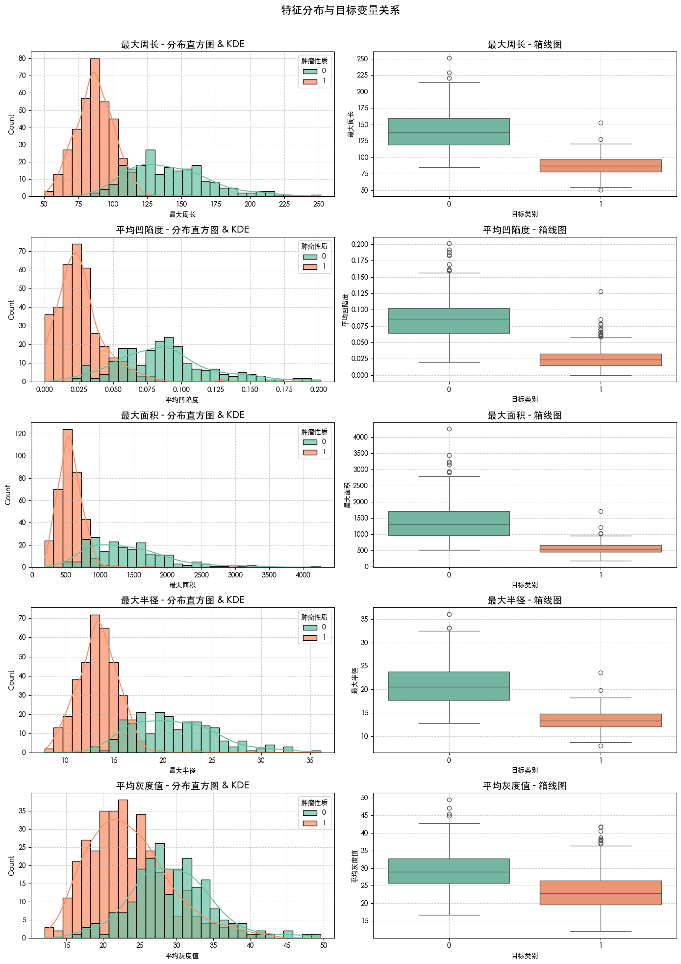
可以发现 数据呈现右偏 应该是使用对数变换处理 不过为了更具体我们测试各类预处理方案
1 | from sklearn.naive_bayes import GaussianNB |
原始: 0.9711
标准化: 0.9651
鲁棒缩放: 0.9651
对数变换: 0.9692
发现不进行预处理反而会更好
朴素贝叶斯
1 | from sklearn.naive_bayes import GaussianNB |
准确率:0.9649
| 实际 \ 预测 | 0 | 1 |
|---|---|---|
| 0 | 39 | 3 |
| 1 | 1 | 71 |
| 类别 | Precision | Recall | F1-Score | Support |
|---|---|---|---|---|
| 0 | 0.97 | 0.93 | 0.95 | 42 |
| 1 | 0.96 | 0.99 | 0.97 | 72 |
| accuracy | 0.96 | 114 | ||
| macro avg | 0.97 | 0.96 | 0.96 | 114 |
| weighted avg | 0.97 | 0.96 | 0.96 | 114 |
逻辑回归
其他的数据我们添加异常值的
1 | df = pd.read_excel('肿瘤数据.xlsx') |
1 | from sklearn.linear_model import LogisticRegression |
准确率:0.9561
| 实际 \ 预测 | 0 | 1 |
|---|---|---|
| 0 | 39 | 3 |
| 1 | 2 | 70 |
| 类别 | Precision | Recall | F1-Score | Support |
|---|---|---|---|---|
| 0 | 0.95 | 0.93 | 0.94 | 42 |
| 1 | 0.96 | 0.97 | 0.97 | 72 |
| accuracy | 0.96 | 114 | ||
| macro avg | 0.96 | 0.95 | 0.95 | 114 |
| weighted avg | 0.96 | 0.96 | 0.96 | 114 |
决策树
1 | from sklearn.tree import DecisionTreeClassifier |
准确率:0.9211
| 实际 \ 预测 | 0 | 1 |
|---|---|---|
| 0 | 37 | 5 |
| 1 | 4 | 68 |
| 类别 | Precision | Recall | F1-Score | Support |
|---|---|---|---|---|
| 0 | 0.90 | 0.88 | 0.89 | 42 |
| 1 | 0.93 | 0.94 | 0.94 | 72 |
| accuracy | 0.92 | 114 | ||
| macro avg | 0.92 | 0.91 | 0.91 | 114 |
| weighted avg | 0.92 | 0.92 | 0.92 | 114 |
XGBoost
1 | from xgboost import XGBClassifier |
XGB Accuracy: 0.9561
| 实际 \ 预测 | 0 | 1 |
|---|---|---|
| 0 | 39 | 3 |
| 1 | 2 | 70 |
| 类别 | Precision | Recall | F1-Score | Support |
|---|---|---|---|---|
| 0 | 0.95 | 0.93 | 0.94 | 42 |
| 1 | 0.96 | 0.97 | 0.97 | 72 |
| accuracy | 0.96 | 114 | ||
| macro avg | 0.96 | 0.95 | 0.95 | 114 |
| weighted avg | 0.96 | 0.96 | 0.96 | 114 |
随机森林
1 | from sklearn.ensemble import RandomForestClassifier |
Random Forest Accuracy: 0.9561
| 实际 \ 预测 | 0 | 1 |
|---|---|---|
| 0 | 39 | 3 |
| 1 | 2 | 70 |
| 类别 | Precision | Recall | F1-Score | Support |
|---|---|---|---|---|
| 0 | 0.95 | 0.93 | 0.94 | 42 |
| 1 | 0.96 | 0.97 | 0.97 | 72 |
| accuracy | 0.96 | 114 | ||
| macro avg | 0.96 | 0.95 | 0.95 | 114 |
| weighted avg | 0.96 | 0.96 | 0.96 | 114 |
- Title: 商业数据分析--肿瘤数据
- Author: 姜智浩
- Created at : 2025-09-23 11:45:14
- Updated at : 2025-09-23 19:48:58
- Link: https://super-213.github.io/zhihaojiang.github.io/2025/09/23/20250923商业数据分析--肿瘤数据/
- License: This work is licensed under CC BY-NC-SA 4.0.