移动房车险购买倾向预测分析

保险已成为“高净值人士”的青睐之选。在当前投资机会较少、股市/楼市/实体经济风险较高的背景下,保险业迎来蓬勃发展,大量保险公司推出人寿型、医疗型、投资理财型等产品,竞争激烈。传统的保险模型往往依赖于历史数据和经验法则,易出现险种推荐错配、过度推销等问题,引发客户信任危机和抵触情绪,损害企业品牌信誉。
本案例旨在通过机器学习技术分析家庭购买保险的历史数据,帮助保险公司更好地理解客户的购买行为和风险偏好。完成数据清洗、特征选择、模型构建、模型评估、模型优化和模型解释等数据分析任务,挖掘影响客户购买移动放车险的重要因素,构建移动房车险购买倾向预测模型,提升推荐准确度,从而在竞争激烈的市场中获得优势。
基本库导入
1 | import pandas as pd |
数据读取
1 | df = pd.read_excel('train.xlsx') |
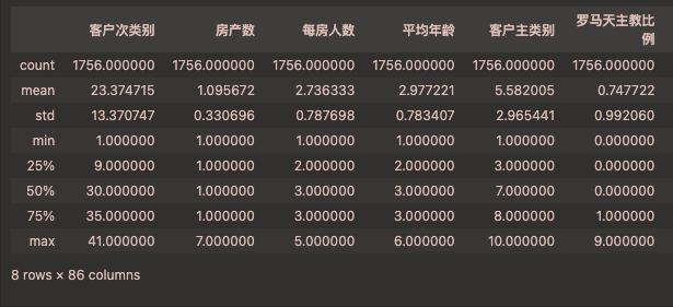
1 | df.info() |
<class ‘pandas.core.frame.DataFrame’>
RangeIndex: 1756 entries, 0 to 1755
Data columns (total 86 columns):Column Non-Null Count Dtype
0 客户次类别 1756 non-null int64
1 房产数 1756 non-null int64
2 每房人数 1756 non-null int64
3 平均年龄 1756 non-null int64
4 客户主类别 1756 non-null int64
5 罗马天主教比例 1756 non-null int64
6 新教比例 1756 non-null int64
7 其它宗教比例 1756 non-null int64
8 无宗教比例 1756 non-null int64
9 已婚占比 1756 non-null int64
10 同居占比 1756 non-null int64
11 其它关系占比 1756 non-null int64
12 单身占比 1756 non-null int64
13 无子女 1756 non-null int64
14 有子女 1756 non-null int64
15 高等教育 1756 non-null int64
16 中等教育 1756 non-null int64
17 低等教育 1756 non-null int64
18 高管 1756 non-null int64
19 企业家 1756 non-null int64
…
84 投保社会安全险数量 1756 non-null int64
85 移动房车险数量 1756 non-null int64
dtypes: int64(86)
memory usage: 1.2 MB(1756, 86)

1 | sns.countplot(x='移动房车险数量', data=df, palette=colors) |
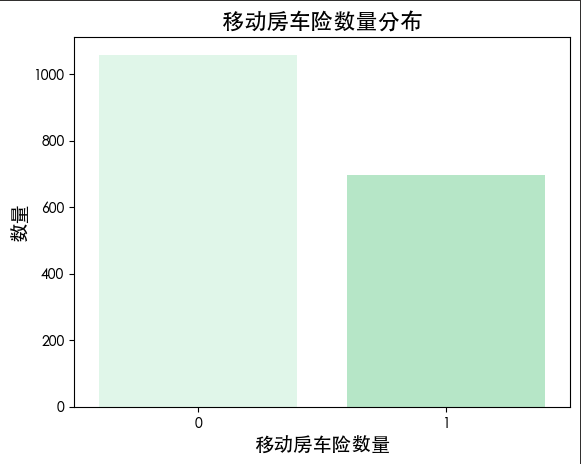
我们查看训练集数据的分布 发现其数量较均匀(也查看了测试集的分布 其购买保险的人数远少于未买保险的人数)
数据清洗
缺失值处理
1 | df.isnull().sum() |
存在缺失值的列:
Index([], dtype=’object’)
发现数据中没有缺失值
异常值处理
检测数据分布
1 | import pandas as pd |
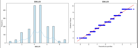
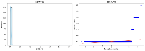
我们可视化了各个特征的分布 发现在前半部份的特征(非投保)数据分布较为正常 在投保部分的特征 数据呈现非常明显的偏态分布 这种情况在进行异常检测时可能是异常值 但考虑到我们这个数据集是预测移动房车险购买倾向 有可能这些异常值就是那些购买保险的人 因此我们可以标记异常值
1 | for col in df.columns: |
特征选择
我们计算方差和皮尔逊相关系数 删除方差过小的特征和p>0.05的特征
1 | low_var = df.var(numeric_only=True) |
[‘客户次类别’, ‘每房人数’, ‘客户主类别’, ‘新教比例’, ‘无宗教比例’, ‘已婚占比’, ‘同居占比’, ‘其它关系占比’, ‘单身占比’, ‘高等教育’, ‘中等教育’, ‘低等教育’, ‘高管’, ‘农场主’, ‘中层管理者’, ‘技术工人’, ‘非熟练劳工’, ‘社会阶层A’, ‘社会阶层B1’, ‘社会阶层C’, ‘社会阶层D’, ‘租房子’, ‘房主’, ‘一辆车’, ‘无车’, ‘公共社保’, ‘私人社保’, ‘收入低于30’, ‘收入45-75’, ‘收入75-122’, ‘平均收入’, ‘购买力水平’, ‘个人第三方保险’, ‘投保车险’, ‘投保机动自行车险’, ‘投保身残险’, ‘投保火险’, ‘投保船险’, ‘投保社会安全险’, ‘第三方私人险数量’, ‘投保车险数量’, ‘投保寿险数量’, ‘投保火险数量’, ‘移动房车险数量’, ‘社会阶层D_outlier’]
剩余变量数量: 45
1 | selected_cols = df.columns.tolist() |
数据划分
1 | X = df.drop(columns=['移动房车险数量']) |
模型构建
我们使用了两种模型处理并优化 第一个使用了朴素贝叶斯模型 使用网格优化 得到
recall=0.73 f1=0.67
相较与只使用朴素贝叶斯 其召回率提高了5%
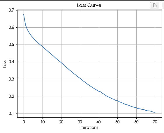
我们又使用多层感知机进行训练并用adam进行优化并且设置了早停 其准确率和召回率达到了0.95和0.96 并且我们更关注模型预测会购买保险的召回率:0.98 说明模型了解了购买保险人的画像
1 | from sklearn.pipeline import Pipeline |
准确率: 0.6822323462414579
召回率: 0.617816091954023
分类报告:
precision recall f1-score support
       0       0.74      0.72      0.73      1060
       1       0.60      0.62      0.61       696

accuracy                           0.68      1756
macro avg      0.67      0.67      0.67      1756
weighted avg   0.68      0.68      0.68      1756
1 | from sklearn.pipeline import Pipeline |
最佳参数: {‘nb__alpha’: 0.1, ‘nb__binarize’: 0.0, ‘nb__class_prior’: [0.4, 0.6]}
最佳模型得分: 0.6235479451448764
分类报告:
precision recall f1-score support
       0       0.78      0.63      0.70      1060
       1       0.57      0.73      0.64       696

accuracy                           0.67      1756
macro avg      0.67      0.68      0.67      1756
weighted avg   0.70      0.67      0.68      1756
1 | from sklearn.pipeline import Pipeline |
准确率: 0.9595671981776766
召回率(宏平均): 0.9635491216655823
分类报告:
precision recall f1-score support
       0       0.99      0.94      0.97      1060
       1       0.92      0.98      0.95       696

accuracy                           0.96      1756
macro avg      0.95      0.96      0.96      1756
weighted avg   0.96      0.96      0.96      1756
特征重要性
1 | import shap |
推荐建议
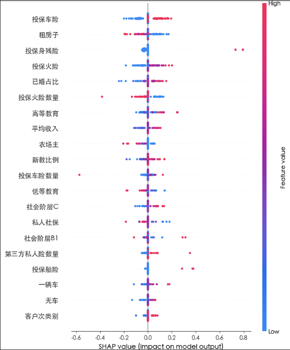
我们使用shap画出了summary_plot
可以看到投保车险 租房子 投保身残险 已婚占比的重要度较高
说明那些会购买移动房车险的客户会给自己的车购买保险 喜欢租房(爱好周游世界)看中自己的生命 已婚
这类人群的用户画像基本可以如此描述:他们喜欢周游世界 有足够的精力去欣赏世界的美好 有着足够的资金去支持自己的爱好
用户群体可能为:退休的老两口 他们的孩子有足够的独立性不需要他们去操心 他们可以安心享受退休生活 他们有着足够的资金去周游世界 去弥补年轻时没空干的事
同时 我们注意到 第三方社会阶层B1 私人险数量和投保船险的影响力较大 虽然在全局中不是特别重要 但是这些也起到关键作用
这类客户的用户画像为40岁以上 公司董事长 其公司十分成熟 在行业内有着举足轻重的地位 其无需担心自己的商业帝国会面临困难 拥有着自己的游艇 为人比较低调 不喜欢显露自己的财富
这类人属于高端客户 他们见过的世面很广 十分精明 虽然数量稀少 但是若成功售出 会给公司带来巨大利润
因此 我们的营销策略为:主要对退休的老两口进行营销 可以在房车经销商处宣发广告 在财经频道 新闻频道宣发广告
同时要打造高端化产品 提供足够的情绪价值 尽可能地打造几个高端的产品以吸引高端客户
- Title: 移动房车险购买倾向预测分析
- Author: 姜智浩
- Created at : 2025-06-05 11:45:14
- Updated at : 2025-06-07 07:29:02
- Link: https://super-213.github.io/zhihaojiang.github.io/2025/06/05/20250607移动房车险购买倾向预测分析/
- License: This work is licensed under CC BY-NC-SA 4.0.