数据来源

https://www.kaggle.com/datasets/rakeshkapilavai/extrovert-vs-introvert-behavior-data/data

数据描述

关于数据集
概述

深入研究“外向与内向性格特征数据集”，这是一个丰富的行为和社交数据集合，旨在探索人类性格谱系。该数据集涵盖了外向和内向的关键指标，是心理学家、数据科学家以及研究社会行为、性格预测或数据预处理技术的研究人员的宝贵资源。

语境

外向和内向等性格特征塑造了个体与社交环境的互动方式。该数据集提供了对个人行为的洞察，例如独处时间、社交活动参与度以及社交媒体参与度，从而为心理学、社会学、市场营销和机器学习等领域的应用提供支持。无论您是预测性格类型还是分析社交模式，该数据集都能助您发现引人入胜的洞见。

数据集详细信息

大小：数据集包含 2,900 行和 8 列。

过程

导入库

import pandas as pd
import numpy as np
import seaborn as sns
import matplotlib.pyplot as plt
%matplotlib inline
from sklearn.model_selection import train_test_split
from sklearn.preprocessing import StandardScaler

查看数据

1	df = pd.read_csv('personality_dataset.csv')

1	df.columns

Index([‘Time_spent_Alone’, ‘Stage_fear’, ‘Social_event_attendance’,
‘Going_outside’, ‘Drained_after_socializing’, ‘Friends_circle_size’,
‘Post_frequency’, ‘Personality’],
dtype=’object’)

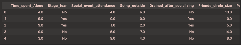
Time_spent_Alone: 独处时间 – 一个人每天通常独自度过的小时数
Stage_fear: 舞台恐惧 – 是否经历过舞台恐惧症
Social_event_attendance: 社交活动出席率 – 参加社交活动的频率（0-10 级）
Going_outside: 外出 – 个人外出的频率（0-10 级）
Drained_after_socializing:社交后精疲力竭 – 社交后是否感觉精疲力尽
Friends_circle_size:好友圈大小 – 亲密朋友数量
Post_frequency:帖子频率 – 在社交媒体上发帖的频率
Personality: 性格 – 目标变量：内向或外向

df.info()

<class ‘pandas.core.frame.DataFrame’>
RangeIndex: 2900 entries, 0 to 2899
Data columns (total 8 columns):

Column Non-Null Count Dtype

0 Time_spent_Alone 2837 non-null float64
1 Stage_fear 2827 non-null object
2 Social_event_attendance 2838 non-null float64
3 Going_outside 2834 non-null float64
4 Drained_after_socializing 2848 non-null object
5 Friends_circle_size 2823 non-null float64
6 Post_frequency 2835 non-null float64
7 Personality 2900 non-null object
dtypes: float64(5), object(3)
memory usage: 181.4+ KB

df.head()

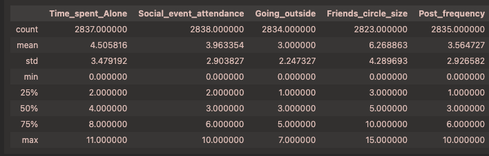
1	df.describe()

缺失值处理

1	df.isnull().sum()

Time_spent_Alone 63
Stage_fear 73
Social_event_attendance 62
Going_outside 66
Drained_after_socializing 52
Friends_circle_size 77
Post_frequency 65
Personality 0
dtype: int64

数值型用均值填充
类别型用众数填充

for col in df.columns:
    if df[col].dtype == 'object':
        df[col] = df[col].fillna(df[col].mode()[0])
    else:
        df[col] = df[col].fillna(df[col].mean())

特征编码

1
2
3

df['Stage_fear'] = df['Stage_fear'].map({'Yes': 1, 'No': 0})
df['Drained_after_socializing'] = df['Drained_after_socializing'].map({'Yes': 1, 'No': 0})
df['Personality'] = df['Personality'].map({'Introvert': 0, 'Extrovert': 1})

异常值检测

for col in df.columns:
    Q1 = df[col].quantile(0.25)
    Q3 = df[col].quantile(0.75)
    IQR = Q3 - Q1
    lower_bound = Q1 - 1.5 * IQR
    upper_bound = Q3 + 1.5 * IQR
    outliers = df[(df[col] >= lower_bound) & (df[col] <= upper_bound)]
    print(f"列{col}的异常值:")

列Time_spent_Alone的异常值:
列Stage_fear的异常值:
列Social_event_attendance的异常值:
列Going_outside的异常值:
列Drained_after_socializing的异常值:
列Friends_circle_size的异常值:
列Post_frequency的异常值:
列Personality的异常值:

说明没有异常值我们通过箱线图也没发现异常值

EDA

工具代码

def pairwise_plot(
    df: pd.DataFrame,
    features: list,
    plot_type: str = 'scatter',  # 可选: 'scatter', 'box', 'bar', 'violin', 'hist'
    hue: str = None,
    max_per_figure: int = 9,
    figsize: tuple = (15, 12),
    fill: bool = None,
    save: bool = False,
    save_prefix: str = "pairplot"
):
    """
    批量绘制特征两两组合的图表，每张大图包含最多9张子图。

    参数:
    - df: DataFrame 数据
    - features: 要组合的特征列名列表
    - plot_type: 图表类型：'scatter', 'box', 'violin', 'hist', 'kde', 'bar'
    - fill: 是否填充 KDE 图（仅适用于 'kde' 类型）
    - hue: 分类变量（可选）
    - max_per_figure: 每页最多显示几个子图
    - figsize: 每张图的整体大小
    - save: 是否保存图像
    - save_prefix: 图像保存的前缀
    """
    import itertools
    import math
    import matplotlib.pyplot as plt
    import seaborn as sns
    combs = list(itertools.combinations(features, 2))
    total_figures = math.ceil(len(combs) / max_per_figure)

    for fig_idx in range(total_figures):
        fig, axs = plt.subplots(3, 3, figsize=figsize)
        axs = axs.flatten()
        start = fig_idx * max_per_figure
        end = start + max_per_figure
        current_combs = combs[start:end]

        for ax_idx, (x, y) in enumerate(current_combs):
            ax = axs[ax_idx]
            if plot_type == 'scatter':
                sns.scatterplot(data=df, x=x, y=y, hue=hue, ax=ax)
            elif plot_type == 'box':
                sns.boxplot(data=df, x=x, y=y, hue=hue, ax=ax)
            elif plot_type == 'violin':
                sns.violinplot(data=df, x=x, y=y, hue=hue, ax=ax)
            elif plot_type == 'bar':
                sns.barplot(data=df, x=x, y=y, hue=hue, ax=ax)
            elif plot_type == 'hist':
                sns.histplot(data=df, x=x, hue=hue, ax=ax, kde=True)
            elif plot_type == 'kde':
                if hue :
                    for label in df[hue].dropna().unique():
                            subset = df[df[hue] == label]
                            sns.kdeplot(data=subset, x=x, y=y, ax=ax, fill=fill, label=str(label), alpha=0.5)
                            ax.legend()
                else:
                    sns.kdeplot(data=df, x=x, y=y, ax=ax, fill=fill)
            else:
                ax.set_title(f"Unsupported plot type: {plot_type}")
            ax.set_title(f"{y} vs {x}")

        # 隐藏多余的子图
        for j in range(len(current_combs), max_per_figure):
            fig.delaxes(axs[j])

        plt.tight_layout()
        if save:
            plt.savefig(f"{save_prefix}_{fig_idx+1}.png", dpi=300)
        plt.show()

可视化

1
2
3

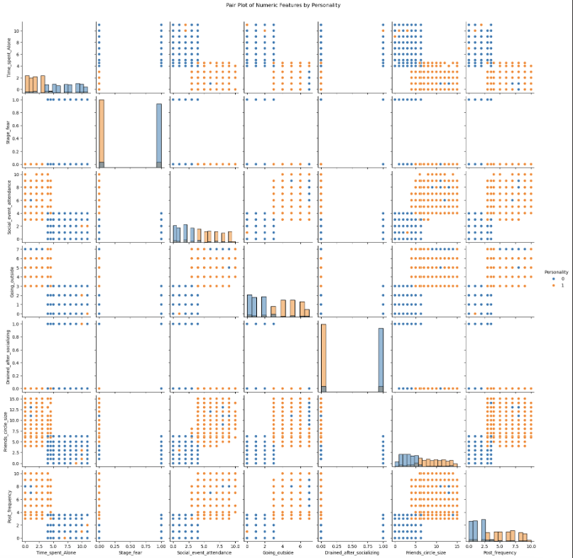
sns.pairplot(df, diag_kind='hist', hue='Personality')
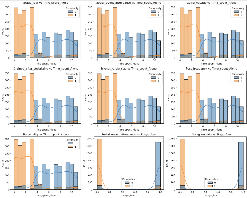
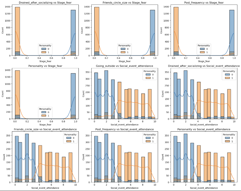
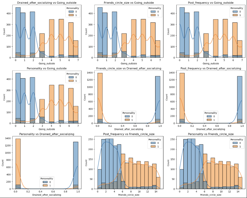
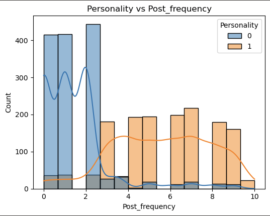
plt.suptitle('Pair Plot of Numeric Features by Personality', y=1.02)
plt.show()

1	pairwise_plot(df, df.columns, plot_type='hist', hue='Personality', max_per_figure=9)

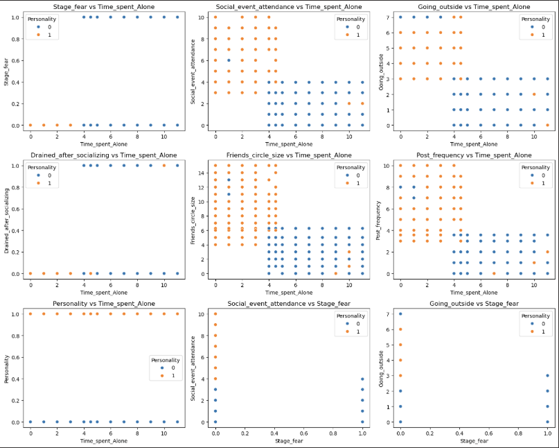
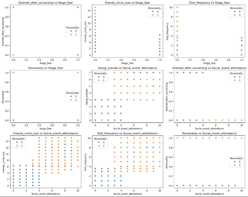
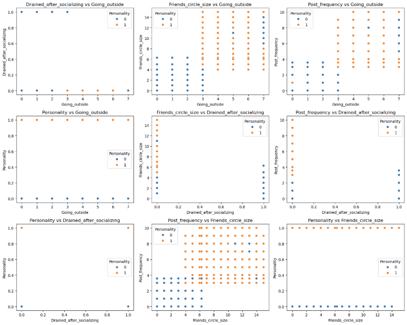
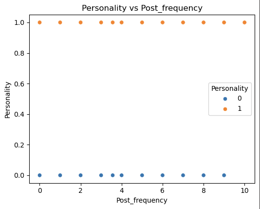
1	pairwise_plot(df, df.columns, plot_type='scatter', hue='Personality', max_per_figure=9)

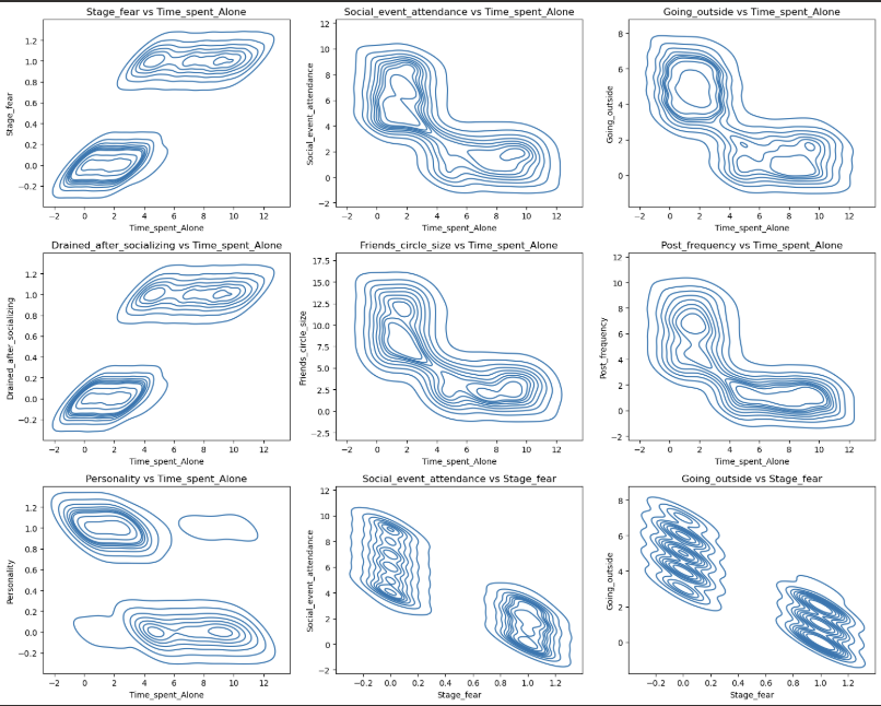
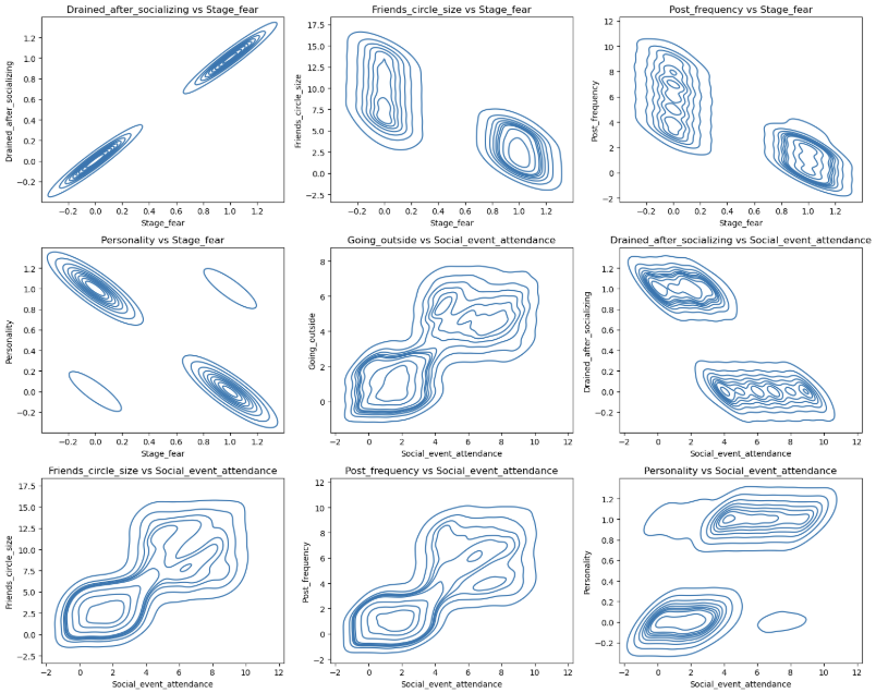
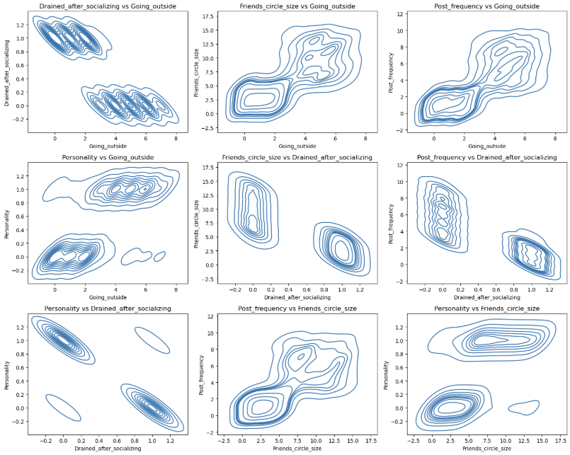
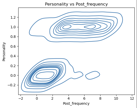
1	pairwise_plot(df, df.columns, plot_type='kde', max_per_figure=9)

df.corr()

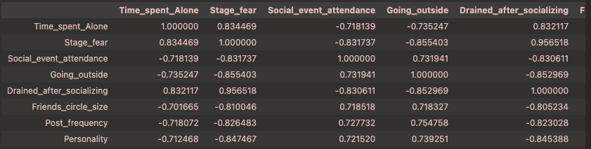
我们发现这些变量与目标变量的相关性的绝对值均大于0.6 说明这些特征都很重要从上面的可视化结果来看也是如此

数据划分

X = df.drop('Personality', axis=1)
y = df['Personality']


X_train, X_test, y_train, y_test = train_test_split(X, y, test_size=0.2, random_state=42)

标准化+模型训练

SVM

from sklearn.pipeline import Pipeline
from sklearn.preprocessing import StandardScaler
from sklearn.svm import SVC
from sklearn.metrics import accuracy_score, classification_report, confusion_matrix

pipeline = Pipeline([
    ('scaler', StandardScaler()),
    ('svm', SVC(kernel='linear'))
])

pipeline.fit(X_train, y_train)

y_pred = pipeline.predict(X_test)
accuracy_score(y_test, y_pred)
report = classification_report(y_test, y_pred)
print(report)
conf_matrix = confusion_matrix(y_test, y_pred)
print(conf_matrix)

0.9293103448275862
precision recall f1-score support
       0       0.92      0.94      0.93       278
       1       0.94      0.92      0.93       302

accuracy                           0.93       580
macro avg 0.93 0.93 0.93 580
weighted avg 0.93 0.93 0.93 580
[[261 17]
[ 24 278]]

from sklearn.pipeline import Pipeline
from sklearn.preprocessing import StandardScaler
from sklearn.svm import SVC
from sklearn.model_selection import GridSearchCV

# 构建Pipeline
pipeline = Pipeline([
    ('scaler', StandardScaler()),
    ('svm', SVC())
])


param_grid = {
    'svm__C': [0.1, 1, 10],
    'svm__kernel': ['linear', 'rbf'],
    'svm__gamma': ['scale', 'auto']
}


grid_search = GridSearchCV(pipeline, param_grid, cv=5)
grid_search.fit(X_train, y_train)


print(grid_search.best_params_)
print(grid_search.best_score_)


y_pred = grid_search.predict(X_test)
report = classification_report(y_test, y_pred)
print(report)
conf_matrix = confusion_matrix(y_test, y_pred)
print(conf_matrix)

{‘svm__C’: 0.1, ‘svm__gamma’: ‘scale’, ‘svm__kernel’: ‘rbf’}
0.9357758620689655
precision recall f1-score support
       0       0.92      0.94      0.93       278
       1       0.94      0.92      0.93       302

accuracy                           0.93       580
macro avg 0.93 0.93 0.93 580
weighted avg 0.93 0.93 0.93 580
[[261 17]
[ 24 278]]

XGboost

from xgboost import XGBClassifier
XGB = XGBClassifier()
XGB.fit(X_train, y_train)

y_pred = XGB.predict(X_test)
print("XGBoost Accuracy:", accuracy_score(y_test, y_pred))
report = classification_report(y_test, y_pred)
print(report)
conf_matrix = confusion_matrix(y_test, y_pred)
print(conf_matrix)

XGBoost Accuracy: 0.9172413793103448
precision recall f1-score support
       0       0.90      0.93      0.91       278
       1       0.93      0.91      0.92       302

accuracy                           0.92       580
macro avg 0.92 0.92 0.92 580
weighted avg 0.92 0.92 0.92 580

[[258 20]
[ 28 274]]

pipeline = Pipeline([
    ('XGB', XGBClassifier(use_label_encoder=False, eval_metric='logloss')),
])

param_grid = {
    'XGB__max_depth': [3, 5, 7],
    'XGB__learning_rate': [0.01, 0.1, 0.2],
    'XGB__n_estimators': [50, 100, 200],
    'XGB__subsample': [0.8, 1.0],
    'XGB__colsample_bytree': [0.8, 1.0],
}


grid_search = GridSearchCV(pipeline, param_grid, cv=5, scoring='recall')
grid_search.fit(X_train, y_train)


print(grid_search.best_params_)
print(grid_search.best_score_)

y_pred = grid_search.predict(X_test)
accuracy = accuracy_score(y_test, y_pred)
print(f"Accuracy: {accuracy}")
report = classification_report(y_test, y_pred)
print(report)
conf_matrix = confusion_matrix(y_test, y_pred)
print(conf_matrix)

Accuracy: 0.9293103448275862
precision recall f1-score support
       0       0.92      0.94      0.93       278
       1       0.94      0.92      0.93       302

accuracy                           0.93       580
macro avg 0.93 0.93 0.93 580
weighted avg 0.93 0.93 0.93 580

[[261 17]
[ 24 278]]

随机森林

from sklearn.ensemble import RandomForestClassifier

rf = RandomForestClassifier(n_estimators=100, random_state=42)
rf.fit(X_train, y_train)

y_pred = rf.predict(X_test)
print("Random Forest Accuracy:", accuracy_score(y_test, y_pred))
report = classification_report(y_test, y_pred)
print(report)
conf_matrix = confusion_matrix(y_test, y_pred)
print(conf_matrix)

Random Forest Accuracy: 0.9224137931034483
precision recall f1-score support
       0       0.91      0.93      0.92       278
       1       0.94      0.91      0.92       302

accuracy                           0.92       580
macro avg 0.92 0.92 0.92 580
weighted avg 0.92 0.92 0.92 580

[[259 19]
[ 26 276]]

pipeline = Pipeline([
    ('rf', RandomForestClassifier(random_state=42)),
])

param_grid = {
    'rf__n_estimators': [50, 100, 200],
    'rf__max_depth': [None, 10, 20, 30],
    'rf__min_samples_split': [2, 5, 10],
    'rf__min_samples_leaf': [1, 2, 4],
}
grid_search = GridSearchCV(pipeline, param_grid, cv=5, scoring='accuracy', n_jobs=-1)
grid_search.fit(X_train, y_train)
best_model = grid_search.best_estimator_

y_pred = best_model.predict(X_test)
accuracy = accuracy_score(y_test, y_pred)
print(f"Best Random Forest Accuracy: {accuracy}")
report = classification_report(y_test, y_pred)
print(report)
conf_matrix = confusion_matrix(y_test, y_pred)
print(conf_matrix)

Best Random Forest Accuracy: 0.9293103448275862
precision recall f1-score support
       0       0.92      0.94      0.93       278
       1       0.94      0.92      0.93       302

accuracy                           0.93       580
macro avg 0.93 0.93 0.93 580
weighted avg 0.93 0.93 0.93 580

[[261 17]
[ 24 278]]

结论

我们通过可视化图表可以看到数据的分布呈现集中分布说明特征与特征之间的关系较为紧密说明内向与外向的人他们具有明显的区分度

SVM的准确率为：0.9357758620689655
预测的召回率为：0.93

其中预测内向的召回率为：0.94
其中预测外向的召回率为：0.92
说明其对内向的确诊率较高

智浩的Blog

Extrovert vs. Introvert Behavior Data