数据来源

https://www.kaggle.com/competitions/playground-series-s5e5/data

数据描述

The dataset for this competition (both train and test) was generated from a deep learning model trained on the Calories Burnt Prediction dataset. Feature distributions are close to, but not exactly the same, as the original. Feel free to use the original dataset as part of this competition, both to explore differences as well as to see whether incorporating the original in training improves model performance.

Files
train.csv - the training dataset; Calories is the continuous target
test.csv - the test dataset; your objective is to predict the Calories for each row
sample_submission.csv - a sample submission file in the correct format.

过程

导入库

import pandas as pd
import numpy as np
import seaborn as sns
import matplotlib.pyplot as plt
%matplotlib inline
from sklearn.model_selection import train_test_split
from sklearn.preprocessing import StandardScaler

查看数据

1 2	df = pd.read_csv('train.csv') df.head()

df.info()

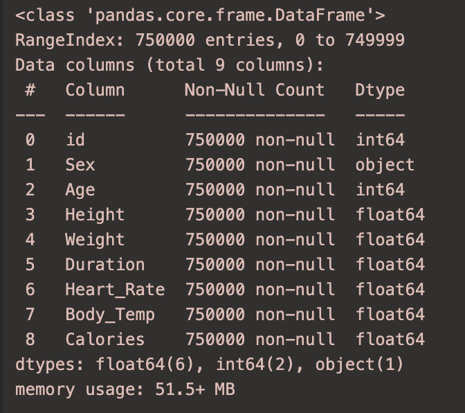
通过翻译得到每个特征的意思：

Sex: 性别，1表示男性，0表示女性
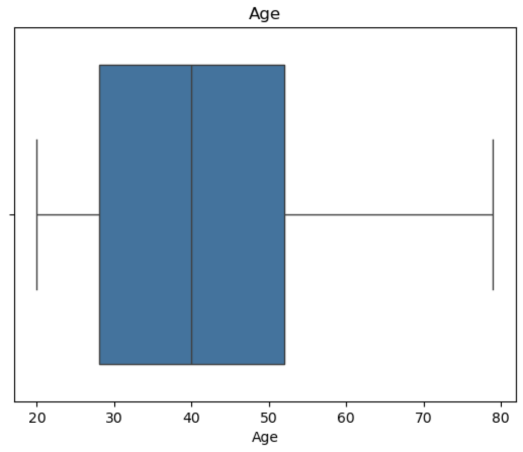
Age: 年龄
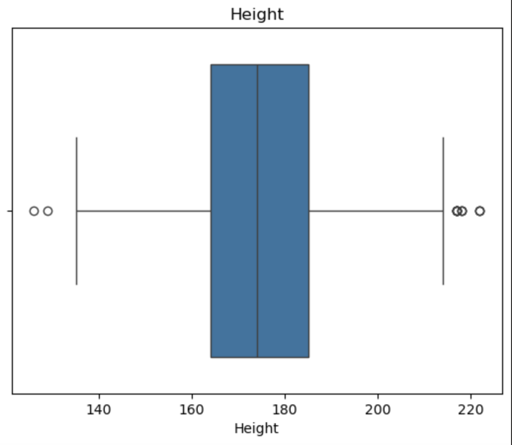
Height: 身高，单位为厘米
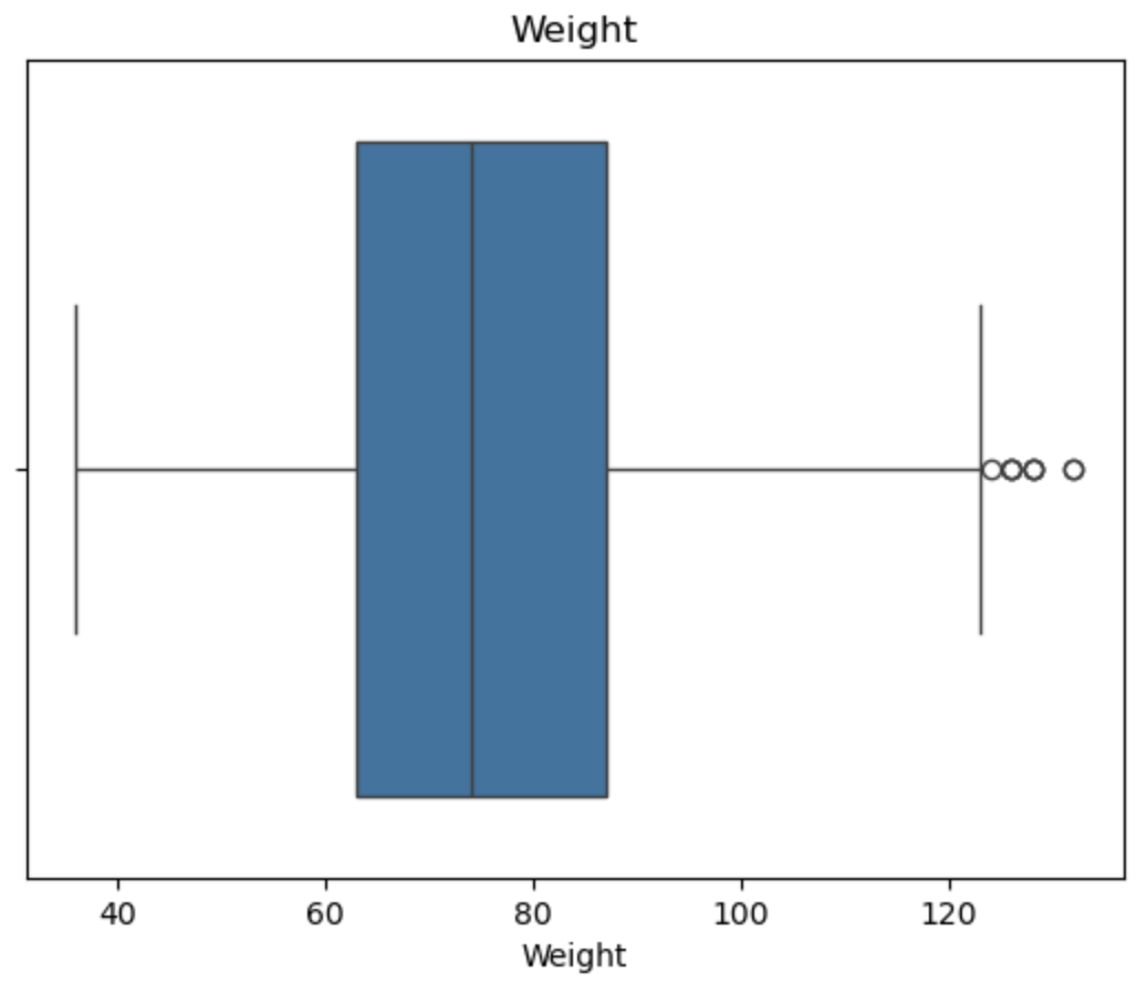
Weight: 体重，单位为千克
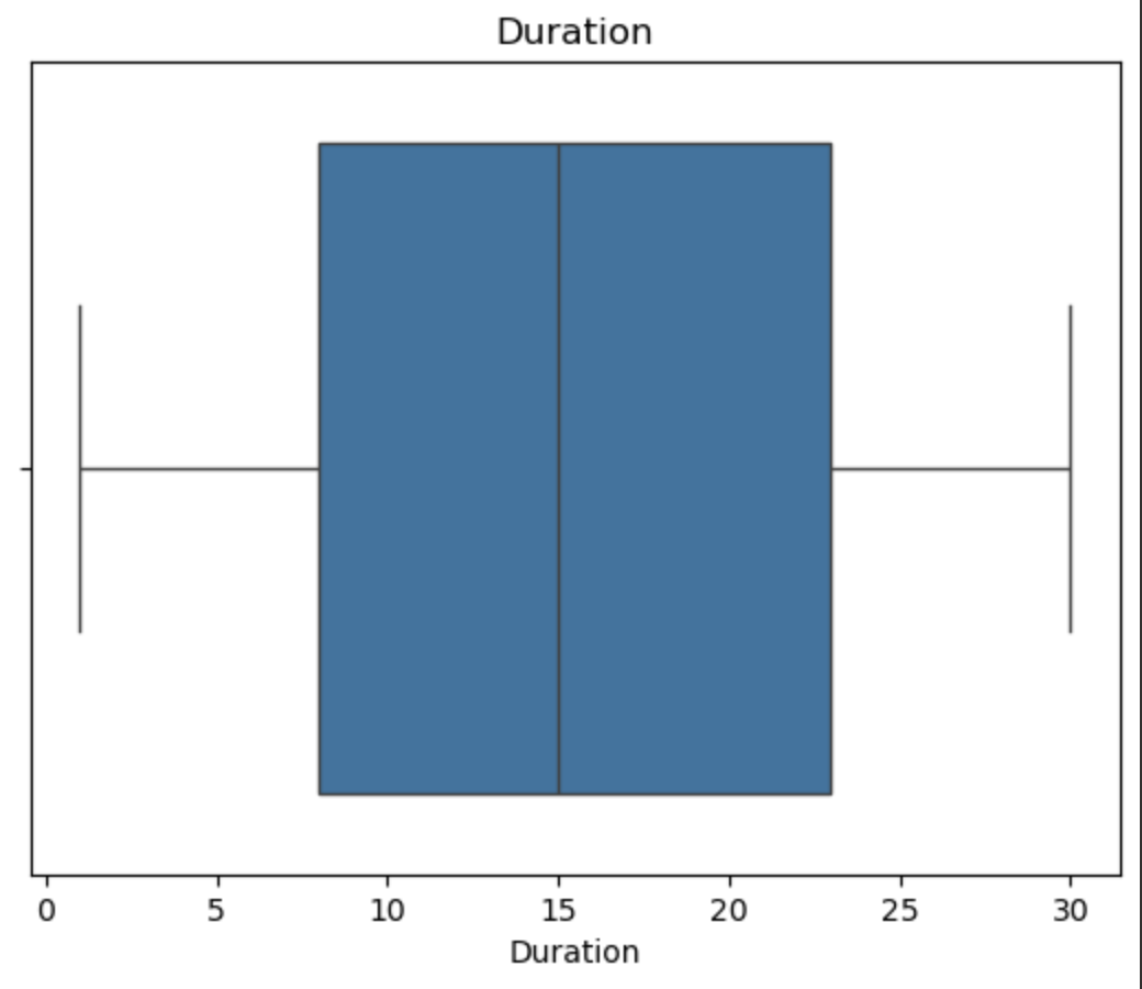
Duration: 活动持续时间，单位为分钟
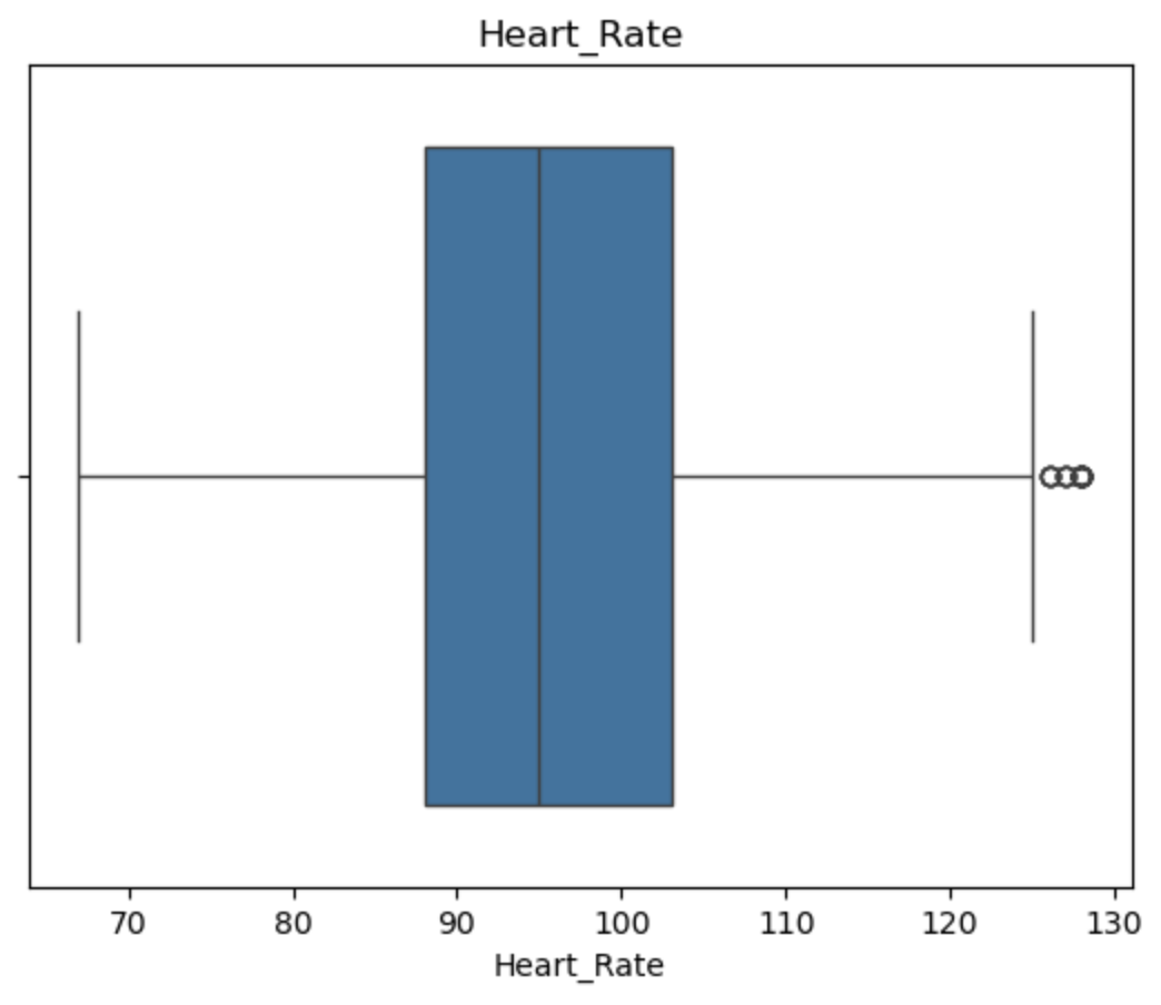
Heart_Rate: 心率，每分钟的心跳次数
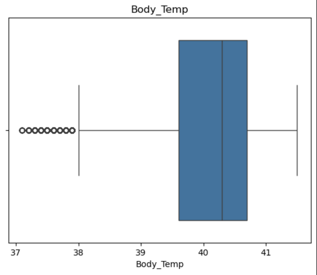
Body_Temp: 体温，单位为摄氏度
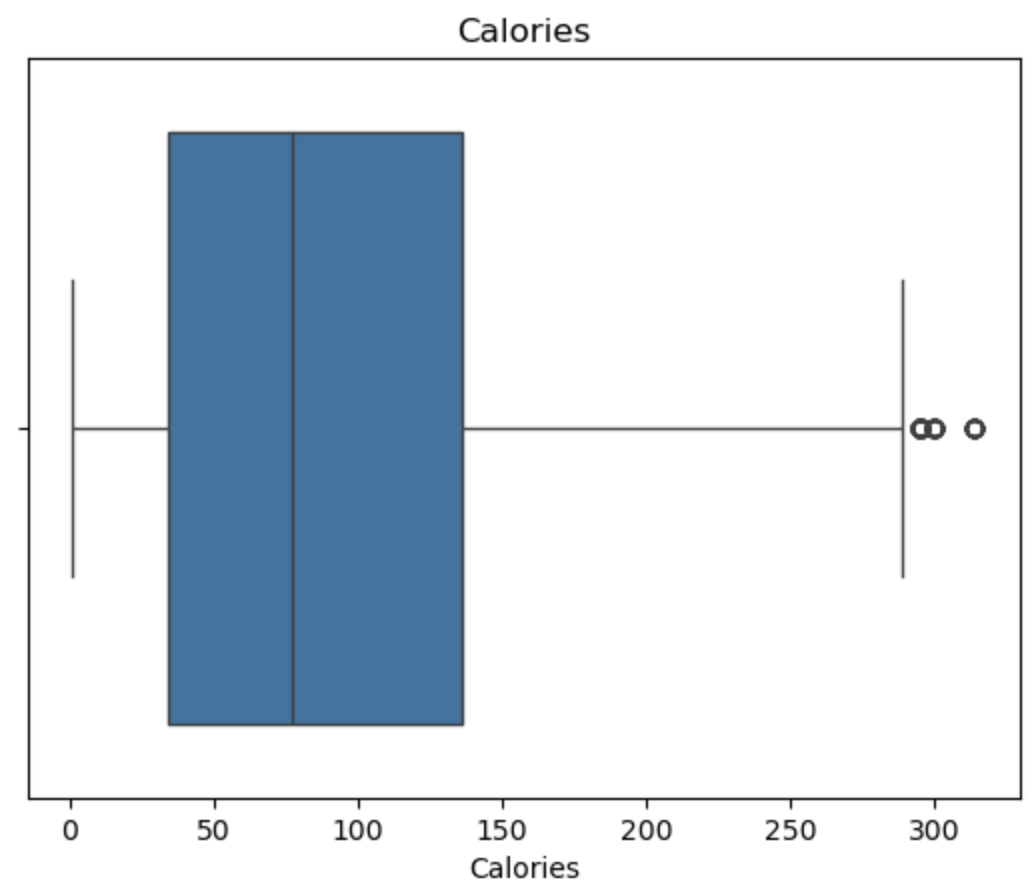
Calories: 卡路里，这是我们要预测的目标变量

我们首先检查数据集中是否存在缺失值

1	df.drop(columns=['id'], inplace=True)

1	df.isnull().sum()

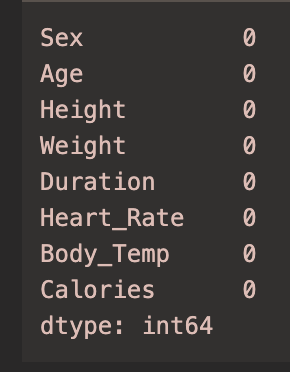
可以看到没有缺失值

由于我们要预测卡路里的消耗量因此我们自然想到BMI这个指标与人体有关因此添加BMI这个特征

1	df['BMI'] = df['Weight'] / (df['Height'] / 100) ** 2

特征编码

将性别转换为数值型

1	df['Sex'] = df['Sex'].replace({'male': 1, 'female': 0})

EDA

for col in df.columns:
    plt.scatter(df[col], df['Calories'])
    plt.xlabel(col)
    plt.ylabel('Calories')
    plt.show()

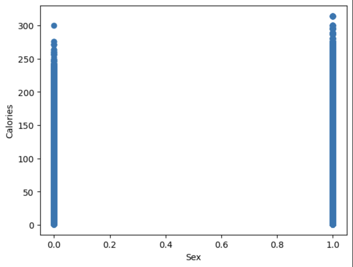
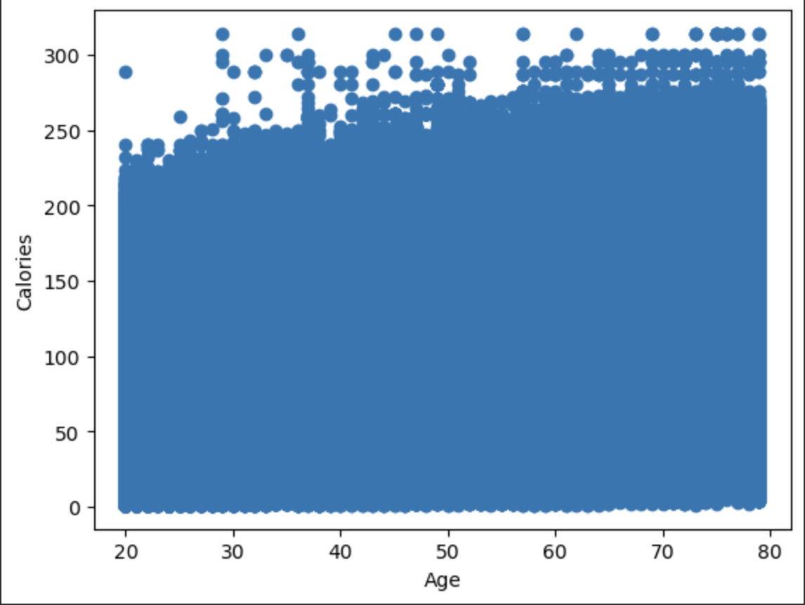
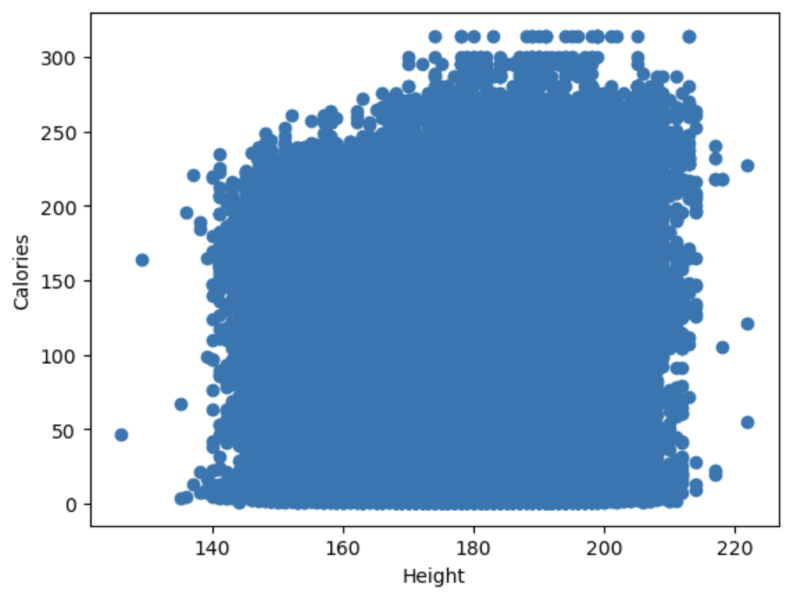
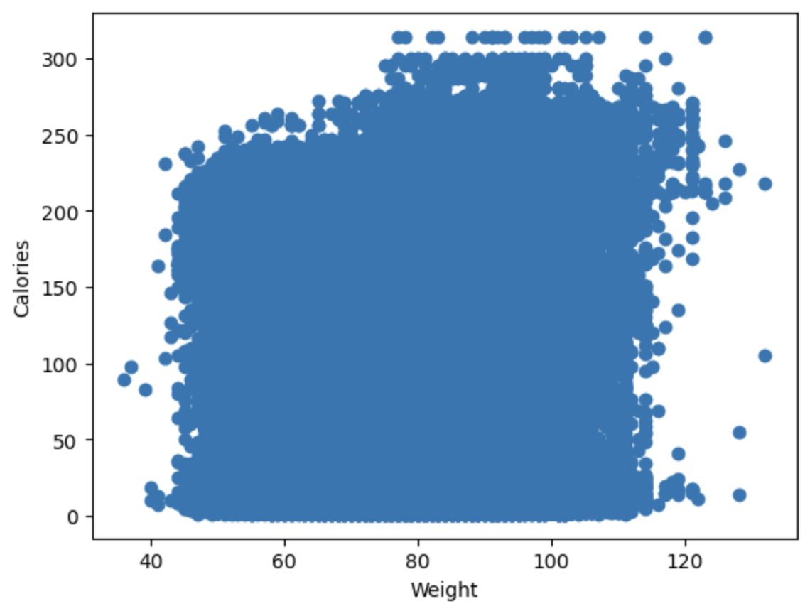
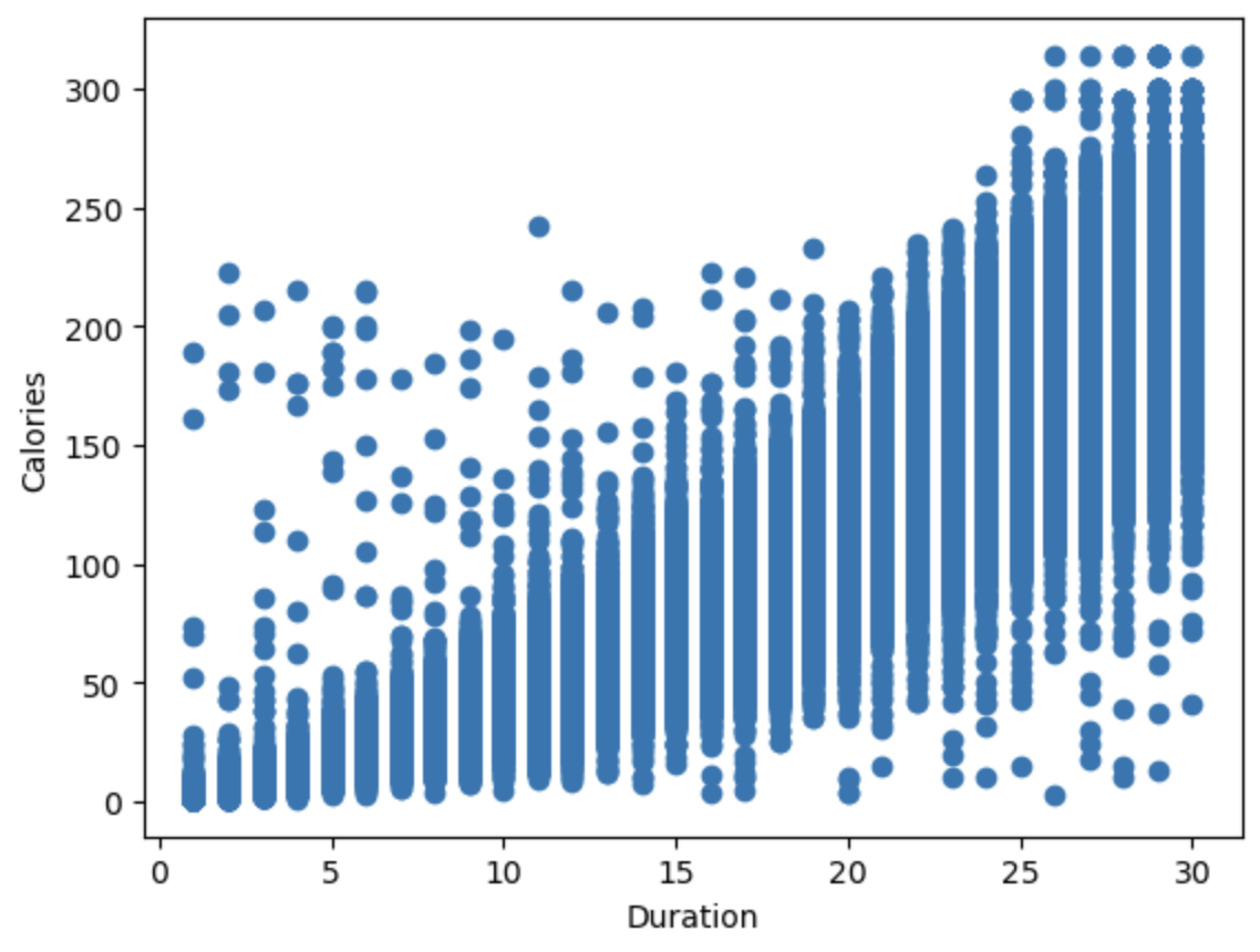
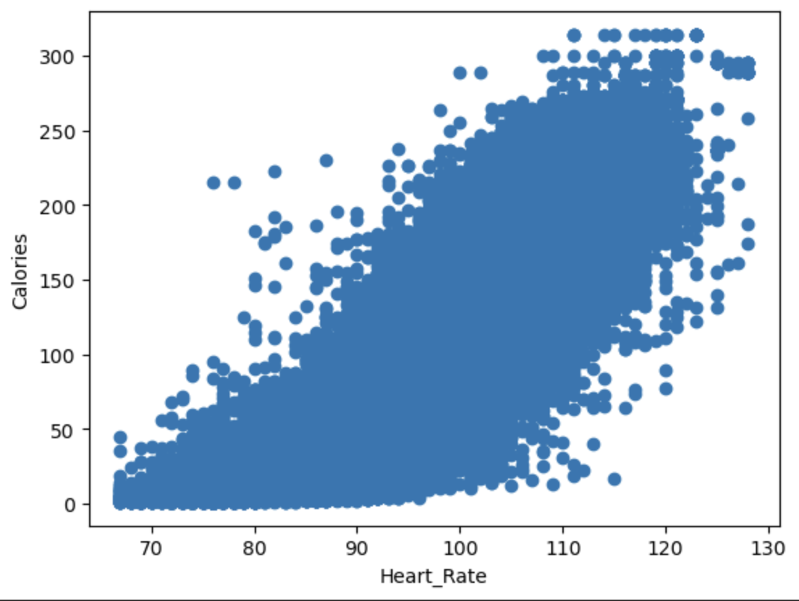
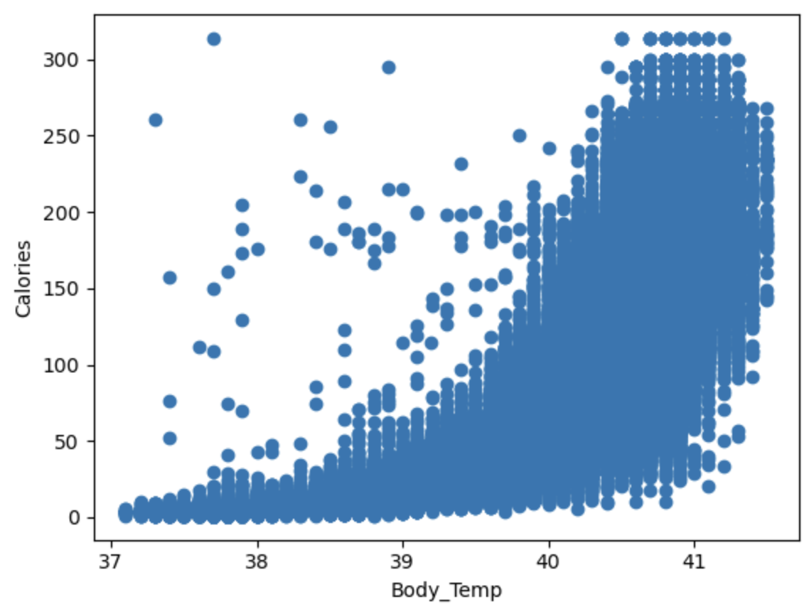
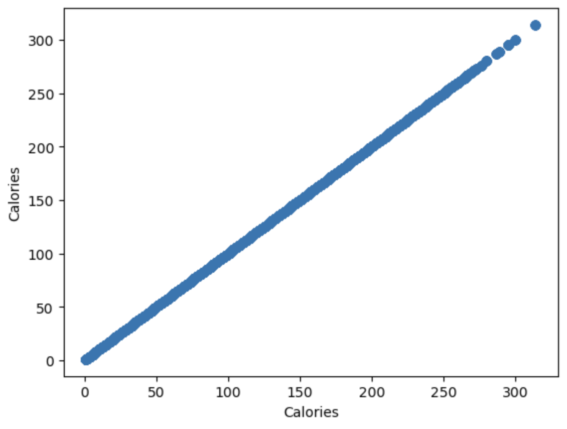
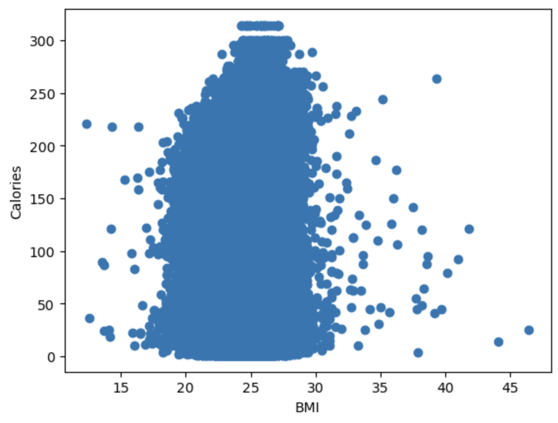
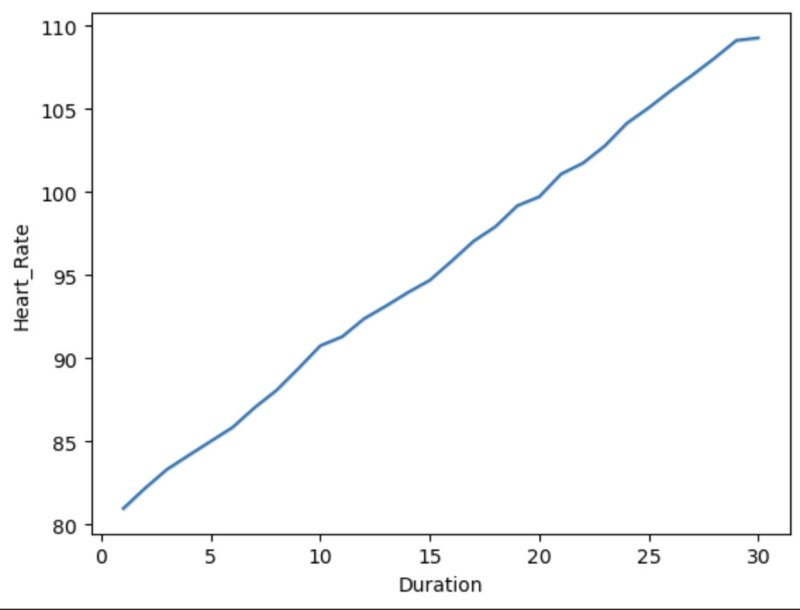
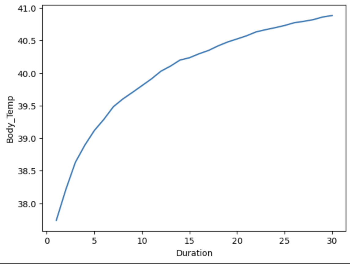
可以看到 duration、Heart_Rate、Body_Temp与Calories呈线性关系
接下来我们查看特征与特征之间的相关性。

1 2	sns.countplot(x=pd.cut(df['Weight'], bins=20, labels=False), data=df,hue='Sex') plt.show()

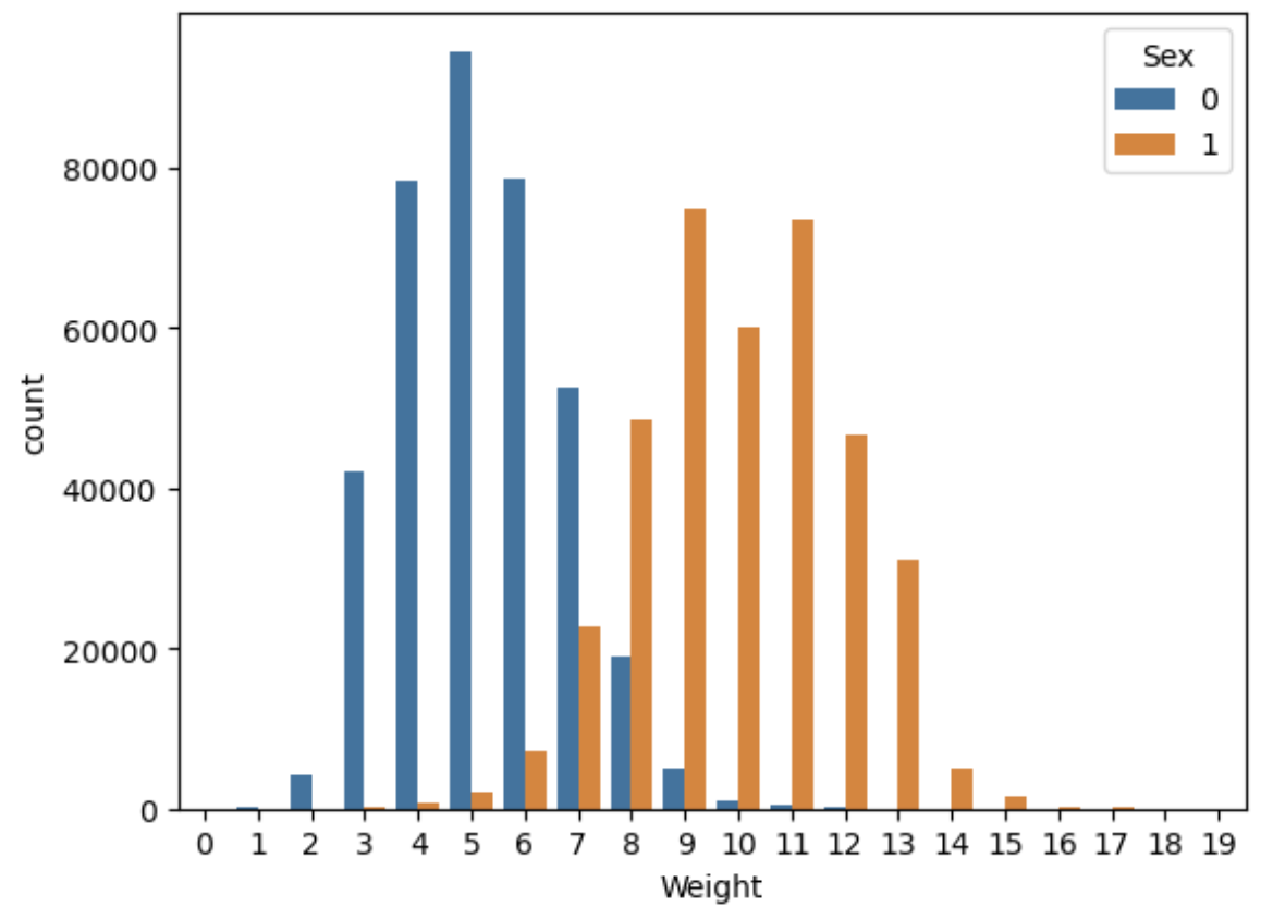
可以看到男性的体重分布是偏右的，而女性的体重分布是偏左的

1 2	sns.lineplot(x='Height',y='Weight',data=df) plt.show()

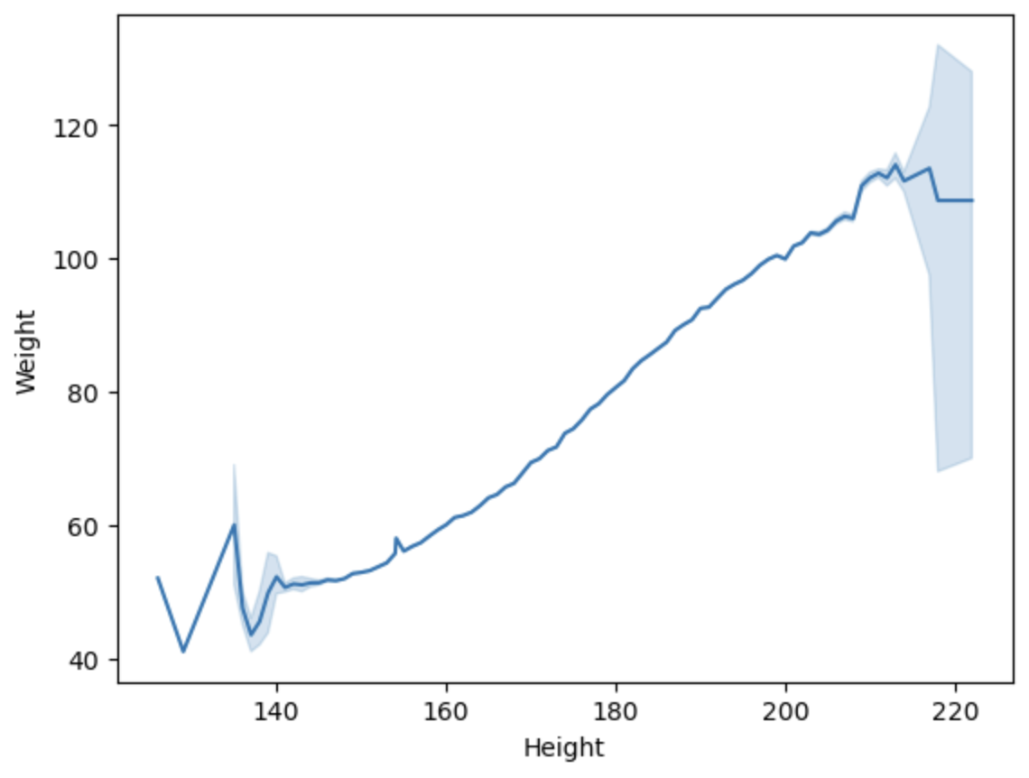
可以看到 Weight与Height存在正相关

1 2	sns.lineplot(x='Duration',y='Heart_Rate',data=df) plt.show()

1 2	sns.lineplot(x='Duration',y='Body_Temp',data=df) plt.show()

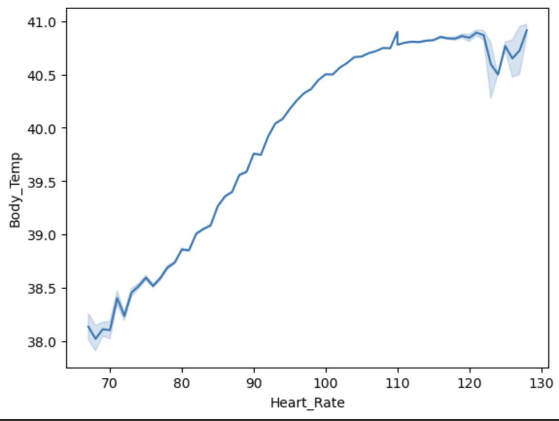
1 2	sns.lineplot(x='Heart_Rate',y='Body_Temp',data=df) plt.show()

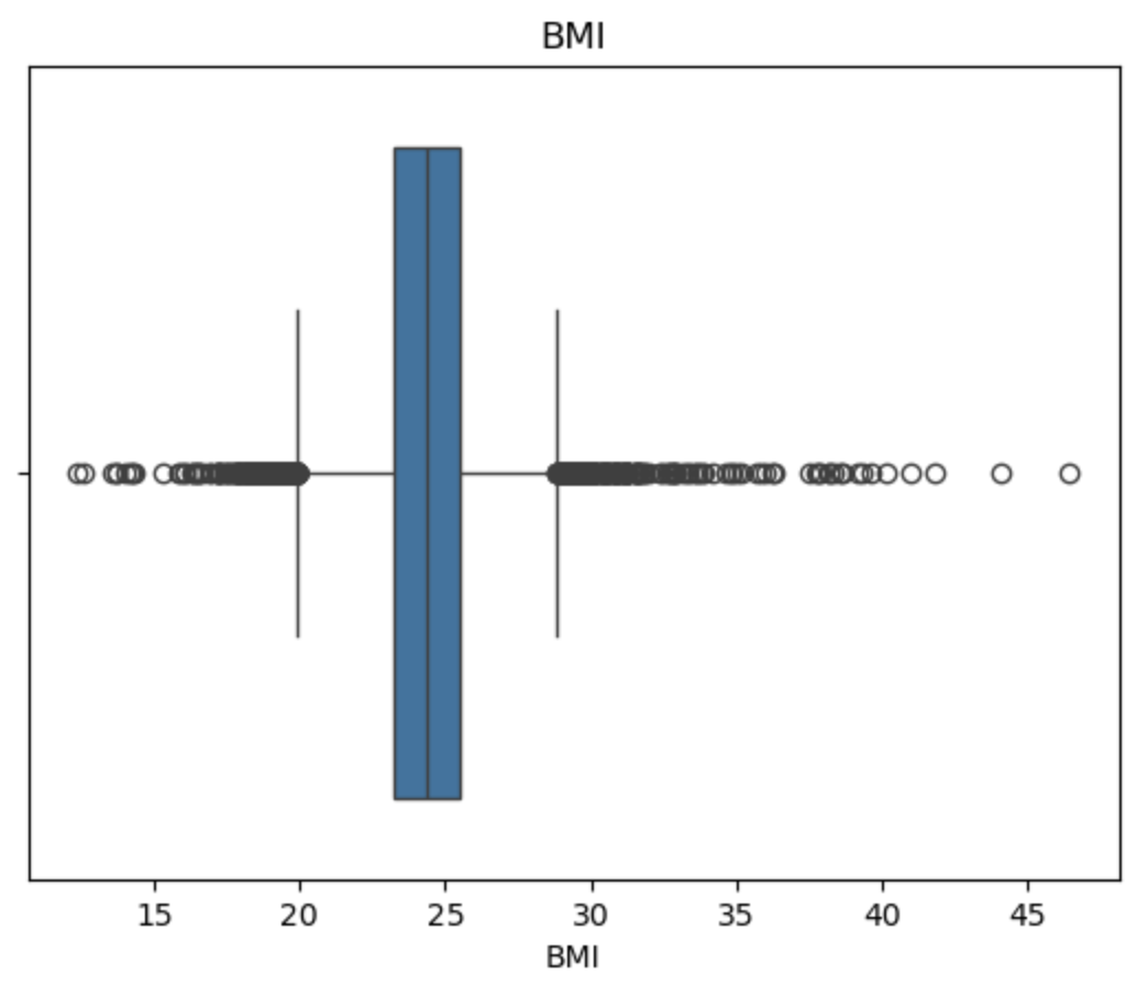
异常值可视化检测

for col in df.columns:
    sns.boxplot(x=df[col])
    plt.title(col)
    plt.show()

from scipy.stats import mstats

features = ['Height', 'Weight', 'Heart_Rate', 'Body_Temp']
for col in features:
    df[col] = mstats.winsorize(df[col], limits=[0.05, 0.05])

特征选择

df.corr()

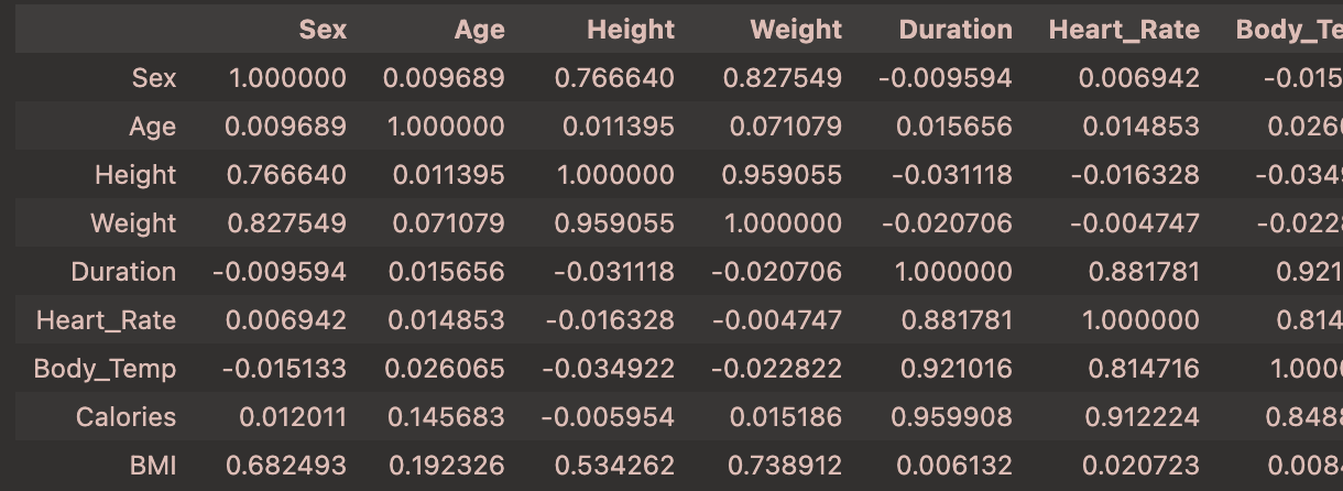
可以看到在相关性分析中

Calories与Duration、Heart_Rate、Body_Temp的相关性最高
为0.959908、0.908748、0.828671，因此选择这三个特征作为模型的输入特征
接下来我们通过卡方检验来选择特征

y = df['Calories']
X = df.drop(['Calories'], axis=1)

X_train, X_test, y_train, y_test = train_test_split(X, y, test_size=0.2, random_state=42)

from sklearn.feature_selection import SelectKBest, chi2

# 使用卡方检验选择前 2 个最佳特征
selector = SelectKBest(chi2, k=3)
X_new = selector.fit_transform(X_train, y_train)
print("选择后的特征形状：", X_new.shape)
print("每个特征的得分：", selector.scores_)
print("是否被选择：", selector.get_support())

# 输出每个特征的得分
scores = pd.Series(selector.scores_, index=X.columns)
scores = scores.sort_values(ascending=False)
print("卡方检验得分最高的特征：\n", scores.head(10))

选择后的特征形状： (600000, 3)
每个特征的得分： [8.72102007e+03 2.13858892e+05 1.32375353e+04 4.71694088e+04
2.61568982e+06 4.35154289e+05 6.94410801e+03 1.65968833e+03]
是否被选择： [False True False False True True False False]
卡方检验得分最高的特征：
Duration 2.615690e+06
Heart_Rate 4.351543e+05
Age 2.138589e+05
Weight 4.716941e+04
Height 1.323754e+04
Sex 8.721020e+03
Body_Temp 6.944108e+03
BMI 1.659688e+03
dtype: float64

1	df.drop(columns=['BMI', 'Sex', 'Weight', 'Height'], inplace=True)

数据划分

y = df['Calories']
X = df.drop(['Calories'], axis=1)

X_train, X_test, y_train, y_test = train_test_split(X, y, test_size=0.2, random_state=42)

scaler = StandardScaler()
X_train_scaled = scaler.fit_transform(X_train)
X_test_scaled = scaler.transform(X_test)

模型选择

from sklearn.linear_model import LinearRegression
from sklearn.ensemble import RandomForestRegressor
import xgboost as xgb
from sklearn.ensemble import GradientBoostingRegressor
from sklearn.metrics import root_mean_squared_error, root_mean_squared_log_error, r2_score

models = {
    'Linear Regression': LinearRegression(),
    'Random Forest': RandomForestRegressor(),
    'XGBoost': xgb.XGBRegressor(),
    'Gradient Boosting': GradientBoostingRegressor()
}

results = []

for name, model in models.items():
    y_train_log = np.log1p(y_train)
    model.fit(X_train_scaled, y_train_log)
    y_pred_log = model.predict(X_test_scaled)
    y_pred = np.expm1(y_pred_log)

    rmse = root_mean_squared_error(y_test, y_pred)
    rmsle = root_mean_squared_log_error(y_test, y_pred)
    r2 = r2_score(y_test, y_pred)
    
    results.append({
        'Model': name,
        'RMSE': rmse,
        'RMSLE': rmsle,
        'R²': r2
    })
results_df = pd.DataFrame(results)
print(results_df)

           Model       RMSE     RMSLE        R²
0 Linear Regression 16.044743 0.212877 0.933576
1 Random Forest 7.287551 0.102109 0.986297
2 XGBoost 6.839083 0.096267 0.987931
3 Gradient Boosting 7.001537 0.097709 0.987351

智浩的Blog

Predict Calorie Expenditure