Predict Podcast Listening Time

数据来源

https://www.kaggle.com/competitions/playground-series-s5e4/data

数据描述

Dataset Description
The dataset for this competition (both train and test) was generated from a deep learning model trained on the Podcast Listening Time Prediction dataset. Feature distributions are close to, but not exactly the same, as the original. Feel free to use the original dataset as part of this competition, both to explore differences as well as to see whether incorporating the original in training improves model performance.

Files
train.csv - the training dataset; Listening_Time_minutes is the target
test.csv - the test dataset; your objective is to predict the Listening_Time_minutes for each row
sample_submission.csv - a sample submission file in the correct format.

过程

导入库

import pandas as pd
import numpy as np
import seaborn as sns
import matplotlib.pyplot as plt
%matplotlib inline
from sklearn.model_selection import train_test_split
from sklearn.preprocessing import StandardScaler
from sklearn.linear_model import LinearRegression
from sklearn.metrics import mean_squared_error,r2_score

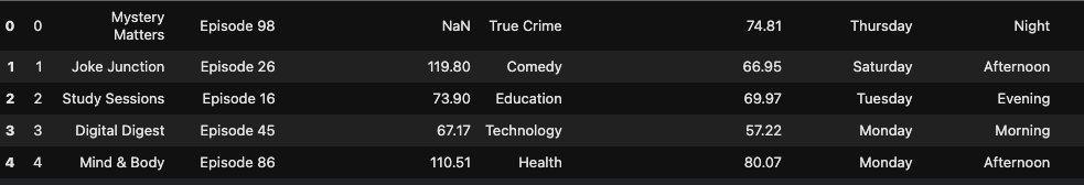
查看数据

1	df = pd.read_csv('/kaggle/input/playground-series-s5e4/train.csv')

df.head()

1	df.describe()

df.info()

现在分析一下这些字段是什么意思：

id：播客名称
podcast_Name：播客名称
Episode_Title：章节标题
Episode_Length_minutes：章节时长
Genre：播客类别
Host_Popularity_percentage：主持人人气百分比
Publication_Day：播放日期
Publication_Time：播放时间
Guest_Popularity_percentage：嘉宾人人气百分比
Number_of_Ads：广告数量
Episode_Sentiment：剧集氛围
Listening_Time_minutes：收听时长 – target

1	df.isnull().sum()

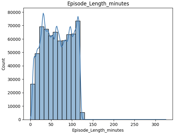
数据可视化

1
2
3

sns.histplot(df['Episode_Length_minutes'], kde=True, bins=30)
plt.title('Episode_Length_minutes')
plt.show()

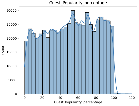
1
2
3

sns.histplot(df['Guest_Popularity_percentage'], kde=True, bins=30)
plt.title('Guest_Popularity_percentage')
plt.show()

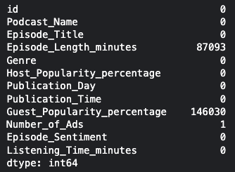
可以看到这两个字段的分布情况比较均匀并且他们都是连续数值型数据利用均值填充

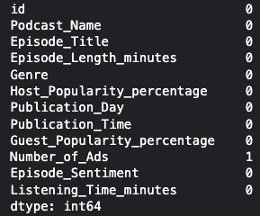
missing_features = ['Episode_Length_minutes', 'Guest_Popularity_percentage']

for feature in missing_features:
    df[feature].fillna(df[feature].mean(), inplace=True)
df.isnull().sum()

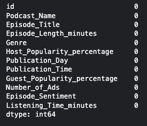
1 2	df.dropna(inplace=True) df.isnull().sum()

接下来我们查看是否存在异常值
利用箱线图来查看是否存在异常值

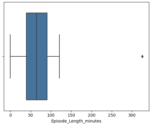
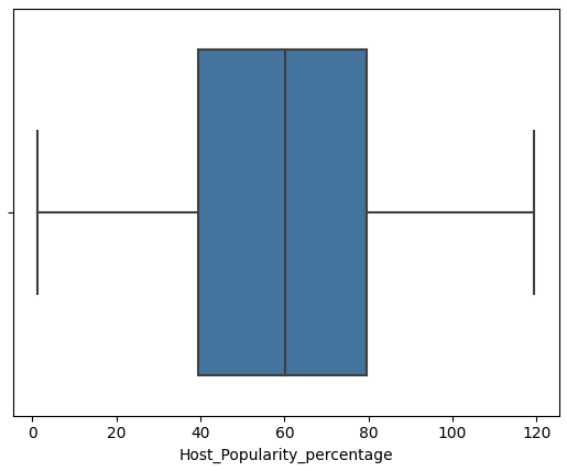
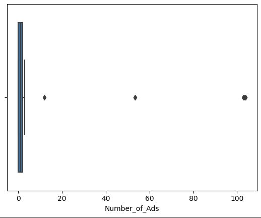
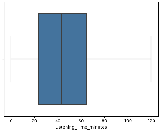
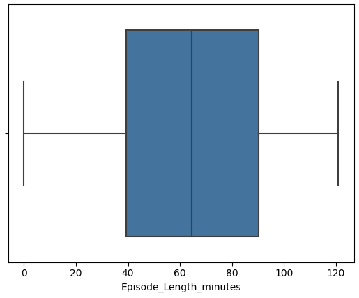
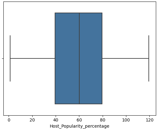
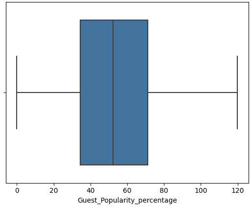
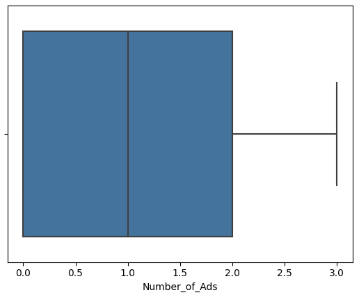
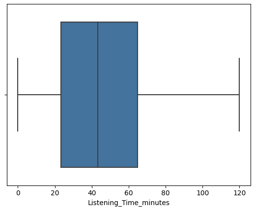
features = ['Episode_Length_minutes', 
            'Host_Popularity_percentage',
        'Guest_Popularity_percentage', 'Number_of_Ads',
    'Listening_Time_minutes']

for col in features:
    sns.boxplot(x=df[col])
    plt.show()

数据预处理

从上述图中可以看到 Episode_Length_minutes和Number_of_Ads存在异常值

Host_Popularity_percentage和Guest_Popularity_percentage存在超过100的值

从常理来看百分比不可能大于100

因此将Episode_Length_minutes和Number_of_Ads的异常值删除

将Host_Popularity_percentage和Guest_Popularity_percentage的异常值进行胜率变换

deleted_features = ['Episode_Length_minutes', 'Number_of_Ads']
df_cleaned = df.copy()

for col in deleted_features:
    Q1 = df_cleaned[col].quantile(0.25)
    Q3 = df_cleaned[col].quantile(0.75)
    IQR = Q3 - Q1

    lower_bound = Q1 - 1.5 * IQR
    upper_bound = Q3 + 1.5 * IQR

    # 只保留当前列在正常范围内的数据（逐步过滤）
    df_cleaned = df_cleaned[(df_cleaned[col] >= lower_bound) & (df_cleaned[col] <= upper_bound)]

检查一遍

features = ['Episode_Length_minutes', 
            'Host_Popularity_percentage',
        'Guest_Popularity_percentage', 'Number_of_Ads',
    'Listening_Time_minutes']

for col in features:
    sns.boxplot(x=df_cleaned[col])
    plt.show()

接下来我们对字符数据进行处理

值得被编码的特征有：

Genre
Publication_Day
Publication_Time
Episode_Sentiment

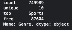
1	df_cleaned['Genre'].describe()

发现他们的类别都较少使用独热编码

from sklearn.preprocessing import OneHotEncoder

one_hot_features = ['Genre', 'Publication_Day', 'Publication_Time', 'Episode_Sentiment']

ohe = OneHotEncoder(sparse_output=False, handle_unknown='ignore')

encoded_array = ohe.fit_transform(df_cleaned[one_hot_features])
encoded_cols = ohe.get_feature_names_out(one_hot_features)

encoded_df = pd.DataFrame(encoded_array, columns=encoded_cols, index=df_cleaned.index)

df_cleaned_encoded = pd.concat([df_cleaned.drop(columns=one_hot_features), encoded_df], axis=1)

1	df_cleaned_encoded.drop(columns=['id', 'Podcast_Name', 'Episode_Title'], inplace=True)

模型选择&模型评估

from sklearn.ensemble import RandomForestRegressor

X = df_cleaned_encoded.drop(columns=['Listening_Time_minutes'])
y = df_cleaned_encoded['Listening_Time_minutes']

X_train, X_test, y_train, y_test = train_test_split(X, y, test_size=0.2, random_state=42)

scaler = StandardScaler()

X_train_scaled = scaler.fit_transform(X_train)
X_test_scaled = scaler.transform(X_test)

rf = RandomForestRegressor(n_estimators=100, random_state=42)
rf.fit(X_train_scaled, y_train)

y_pred = rf.predict(X_test_scaled)

mse = mean_squared_error(y_test, y_pred)
print("Mean Squared Error:", mse)
r2 = r2_score(y_test, y_pred)
print("R^2 Score:", r2)

在我的MacBook AirM2上该模型用时约4‘47秒

Mean Squared Error: 161.35316711251312

R^2 Score: 0.7801317443922687

未进行特征工程

参考来源

chatGPT 4o
提问的问题：

在数据分析中如何查看是否存在缺失值
针对缺失值在什么情况下用均值填充在什么情况下用众数填充在什么情况下用中位数填充
如何对缺失值做可视化图表查看缺失值的分布情况
数据分布比较均匀的其缺失值如何填充
Mean Squared Error: 161.35316711251312 R^2 Score: 0.7801317443922687 这个分数对于一个有29个维度使用随机森林训练的数据来说怎么样
做相关性矩阵就是做个sns.heatmap吗
我对object进行独热编码后对相关性矩阵
这个图看起来很吃力我该怎么做
代码优化：

from sklearn.preprocessing import OneHotEncoder

one_hot_features = ['Genre', 'Publication_Day', 'Publication_Time', 'Episode_Sentiment']
ohe = OneHotEncoder(sparse=False)
for col in one_hot_features:
    df_cleaned_encoded = ohe.fit_transform(pd.DataFrame(col))

---------------------------------------------------------------------------
TypeError                                 Traceback (most recent call last)
Cell In[18], line 4
      1 from sklearn.preprocessing import OneHotEncoder
      3 one_hot_features = ['Genre', 'Publication_Day', 'Publication_Time', 'Episode_Sentiment']
----> 4 ohe = OneHotEncoder(sparse=False)
      5 encoded_parts = []
      6 for col in one_hot_features:

TypeError: OneHotEncoder.__init__() got an unexpected keyword argument 'sparse'

from sklearn.feature_selection import SelectKBest, chi2
from sklearn.datasets import load_iris

# 使用卡方检验选择前 2 个最佳特征
selector = SelectKBest(chi2, k=2)
X_new = selector.fit_transform(X_train, y_train)
print("选择后的特征形状：", X_new.shape)
print("每个特征的得分：", selector.scores_)
print("是否被选择：", selector.get_support())

# 输出每个特征的得分
scores = pd.Series(selector.scores_, index=X.columns)
scores = scores.sort_values(ascending=False)
print("卡方检验得分最高的特征：\n", scores.head(20))

显示报错

ValueError: Unknown label type: (array([48.82398, 72.06621,  0.     , ..., 13.09288, 30.92493, 29.3002 ]),)

from sklearn.decomposition import PCA

# 使用 PCA 降维到 2 维
pca = PCA(n_components=9)
X_pca = pca.fit_transform(X_train)
print("降维后的数据形状：", X_pca.shape)

# 查看每个主成分的贡献率
explained_variance = pd.Series(pca.explained_variance_ratio_, index=[f'PC{i+1}' for i in range(9)])
print("主成分贡献率：\n", explained_variance)

降维后的数据形状： (599991, 9)
主成分贡献率：
 PC1    0.458917
PC2    0.297558
PC3    0.241425
PC4    0.000588
PC5    0.000160
PC6    0.000159
PC7    0.000125
PC8    0.000119
PC9    0.000114

我想查看到底是哪9个特征

我的此项目的kaggle网址：
https://www.kaggle.com/code/super213/randomforest-r-2-0-78

智浩的Blog