机器学习作业笔记

我们需要利用回归分析预测世界大学综合得分
#Jupyter notebook代码
基本库导入
1 | import pandas as pd |
1 | university = pd.read_csv('cwurData.csv') |
此时可能会出现报错
报错信息
File parsers.pyx:574, in pandas._libs.parsers.TextReader.cinit()
File parsers.pyx:663, in pandas._libs.parsers.TextReader._get_header()
File parsers.pyx:874, in pandas._libs.parsers.TextReader._tokenize_rows()
File parsers.pyx:891, in pandas._libs.parsers.TextReader._check_tokenize_status()
File parsers.pyx:2053, in pandas._libs.parsers.raise_parser_error()
File
UnicodeDecodeError: ‘utf-8’ codec can’t decode bytes in position 3864-3865: invalid continuation byte
不用担心,这是因为pd.read_csv()在不指明encoding时默认使用utf-8编码
这段报错是因为该文件不是使用utf-8进行编码。
我们可以写一段代码判断文件的编码格式
1 | import chardet |
之后将其输出的encoding写入pd.read_csv()即可
1 | university = pd.read_csv('cwurData.csv', encoding='GBK') |
输出结果为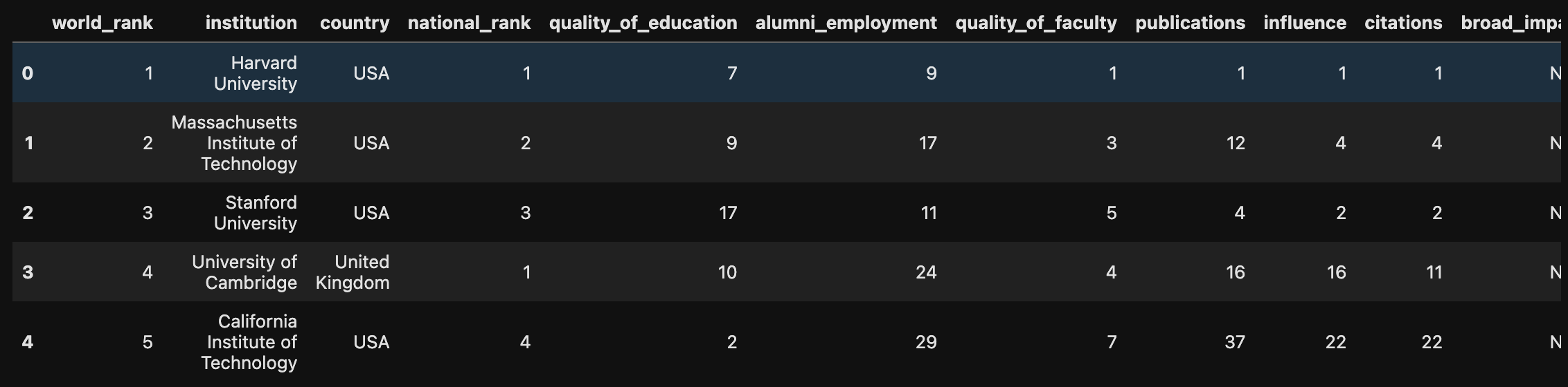
通过该数据可知其数字应该是越小越好
因此相关性应该是负数 且越小越好
之后我们查看文件的维度
1 | university.shape |
输出结果为:(2200, 14)
说明该文件总共有2200行数据,14个特征
接下来我们分析下文件是否有异常
1 | university.describe() |
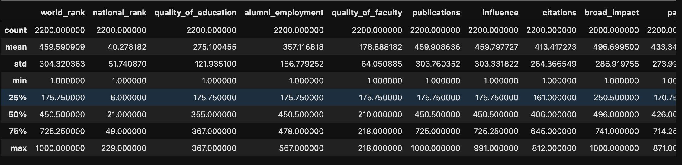
从第一行(count)看到 broad_impact数据与其他数据不同
上述从head()函数我猜测broad_impact列全是NA
仔细查看文件后可知:2012年和2013年的broad_impact存在缺失
其他数据看起来没什么问题 数据质量基本完整
先用相关性矩阵看看各个数据之间的关系
1 | y = university['score'] |
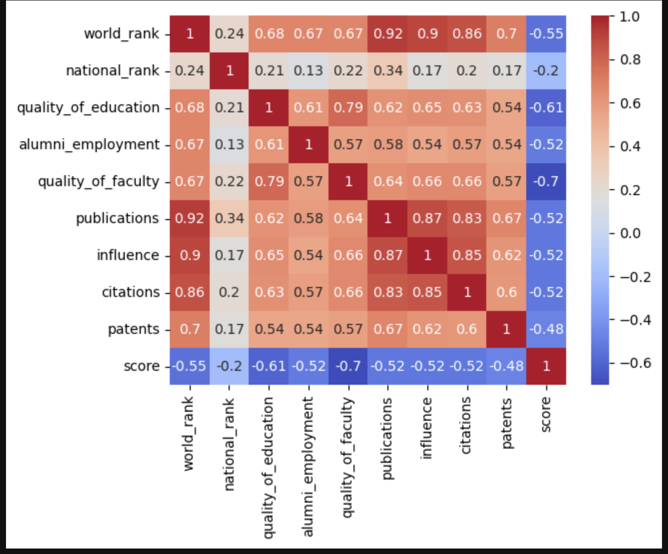
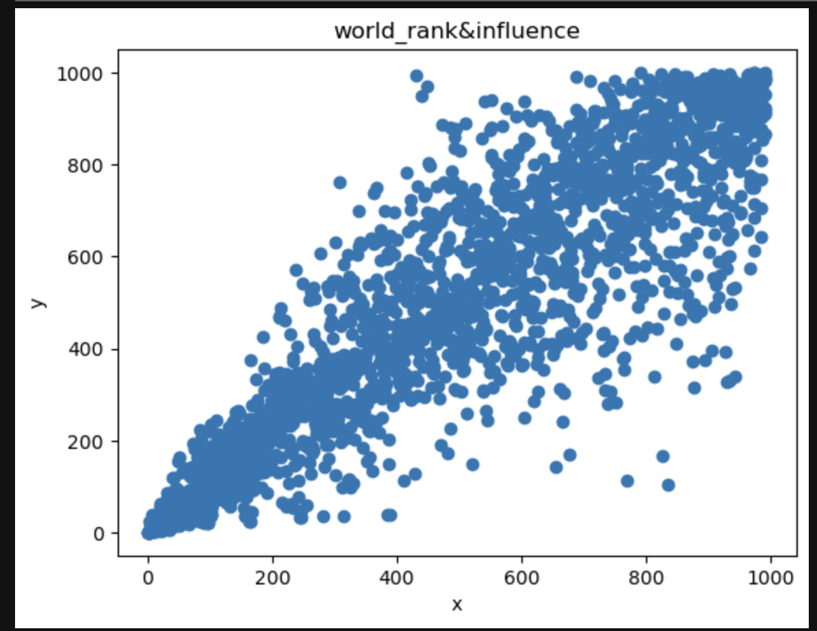
通过上图可以看到world_rank与publications、influence、citations有强相关性
我们用matplotlib.pyplot库做出这些图
1 | x = university["publications"] |
1 | x = university["influence"] |
1 | x = university["citations"] |
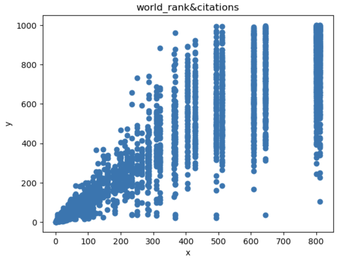
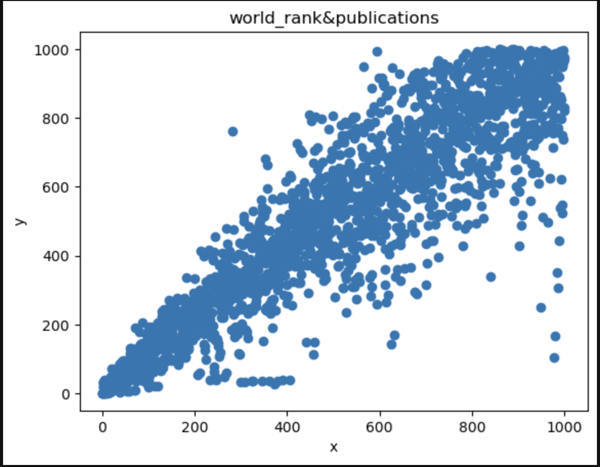
从上述三幅图可以看到world_rank与publications、influence有强相关性
world_rank与citations也有一定的相关性 但不是很明显
再继续做几张图看看其他数据之间的关系怎么样
1 | x = university["publications"] |
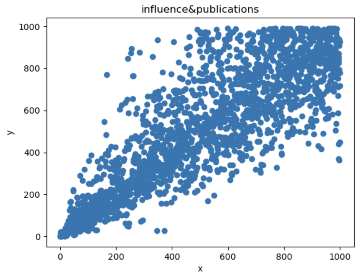
从图中可以看出点近似集中在一条直线上
说明出版物与影响力成正比
1 | x = university["broad_impact"] |
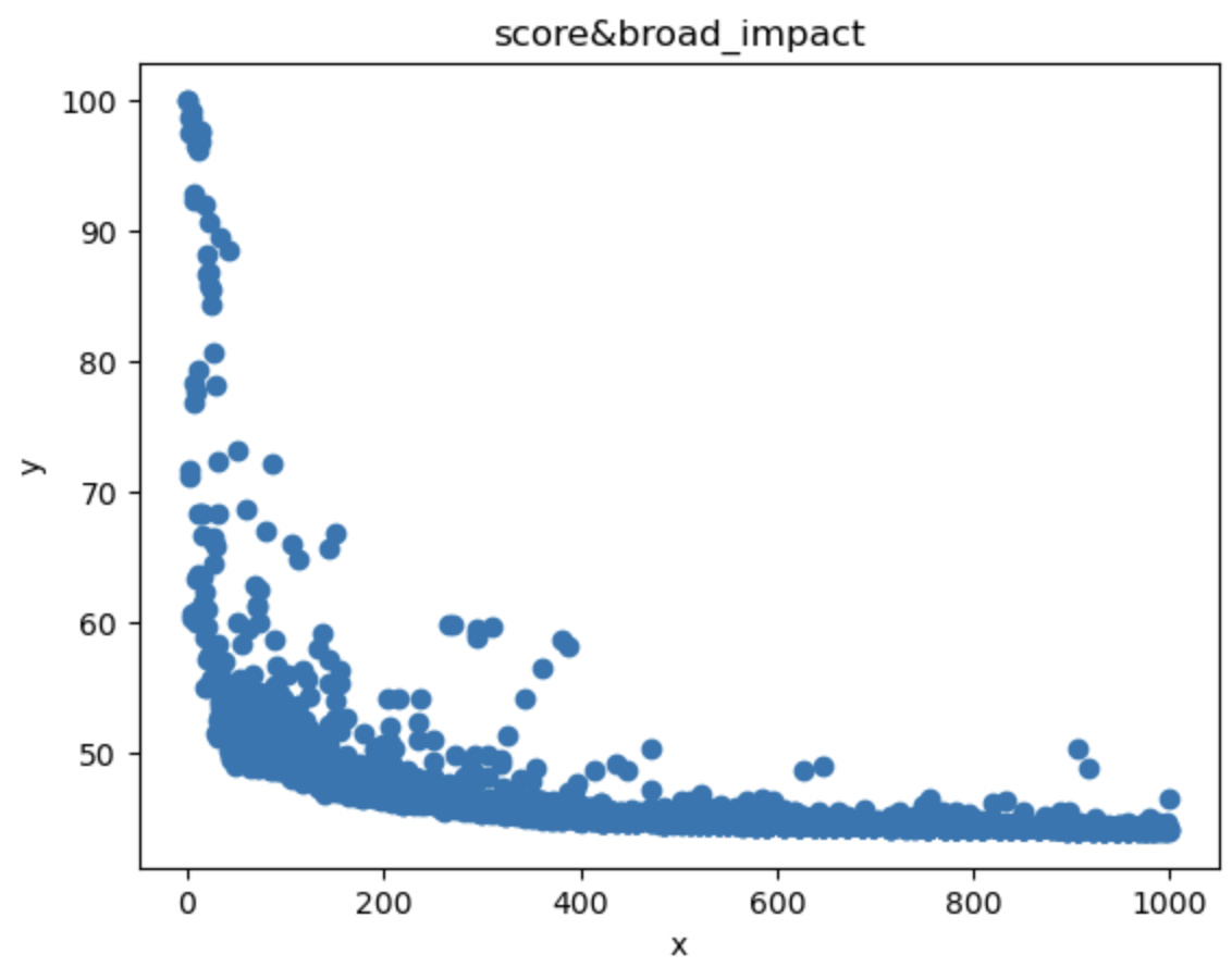
从图中可以看出broad_impact与score成非线性关系 broad_impact的大小与score无关
用相关性进行检测
1 | x = university["broad_impact"] |
输出结果为:r: -0.5315904271503679
呈现负相关 因此确定 broad_impact的大小与score无关
并且broad_impact中存在缺失值
缺失值的处理一般会使用用众数填充、前或后一个数填充、删除缺失列来处理
这里broad_impact的大小与score无关
因此可以将此列删去
同时也可以降低维度
1 | y = university['score'] |
其结果为:
63.60601390140695
world_rank 0.0
national_rank -0.0
quality_of_education -0.0
alumni_employment -0.0
quality_of_faculty -0.0
publications -0.0
influence -0.0
citations -0.0
patents -0.0
dtype: float64
说明模型拟合得不好
查看其均方根误差和决定系数
1 | lr_train_pred = lr.predict(X_train) |
输出结果为:
训练集上的均方根误差和决定系数分别为: 5.441831802594455 0.079429595738992
测试集上的均方根误差和决定系数分别为: 5.369301125131177 0.06344204755145388
上述系数过小可能是数值之间差别过大导致拟合得不好
将其进行标准化
1 | scaler = StandardScaler() |
输出结果为:
world_rank 0.0
national_rank -0.0
quality_of_education -0.0
alumni_employment -1.0
quality_of_faculty -4.0
publications -0.0
influence -0.0
citations -0.0
patents -0.0
dtype: float64
47.83457386363636
模型得到的结果很低 说明拟合得不好
更换其他线性回归模型试试
岭回归
1 | ridge= linear_model.Ridge(alpha=0.05) |
输出结果为:
截距为: 63.60601382257282
回归系数为: [ 0.00116895 -0.00608447 -0.00380894 -0.00592045 -0.06344228 -0.00045937
-0.0009899 -0.00046924 -0.00164281]
RMSE: 5.369301120766853
lasso回归
1 | lasso= linear_model.Lasso(alpha=0.05) |
输出结果为:
截距为: 63.602800047243974
回归系数为: [ 0.00115484 -0.00606551 -0.00381082 -0.00591616 -0.06342471 -0.00045677
-0.00098495 -0.00046729 -0.00164163]
RMSE: 5.369181579518303
弹性网回归
1 | elastic= linear_model.ElasticNet(alpha=0.1,l1_ratio=0.4) |
输出结果为:
截距为: 63.60327653271375
回归系数为: [ 0.00115777 -0.0060693 -0.00381124 -0.00591707 -0.06342543 -0.00045734
-0.00098603 -0.00046779 -0.00164194]
RMSE: 5.369181579518303
可以看到这些回归得到的结果都不好
说明这个不是呈线性关系
我们使用随机森林进行尝试
1 | rf = RandomForestRegressor() |
输出结果为:
训练集上的均方根误差和决定系数分别为: 0.396126717281446 0.9974538720434839
测试集上的均方根误差和决定系数分别为: 1.0185613846393418 0.9808937922886296
可以看到 决定系数为0.99 0.98以上 说明模型拟合得很好
- Title: 机器学习作业笔记
- Author: 姜智浩
- Created at : 2025-03-28 11:45:14
- Updated at : 2025-03-30 14:43:41
- Link: https://super-213.github.io/zhihaojiang.github.io/2025/03/28/20250328机器学习笔记/
- License: This work is licensed under CC BY-NC-SA 4.0.